Ch13: Multiple Testing

import numpy as np
import pandas as pd
import matplotlib.pyplot as plt
import seaborn as sns

sns.set_theme()

%matplotlib inline

import statsmodels.api as sm
from ISLP import load_data
from scipy.stats import ttest_1samp
from statsmodels.stats.multitest import multipletests

Conceptual

Q1.

(a) We expect to get \(\alpha\) Type \(\text{I}\) errors for each of the \(m\) null hypotheses, so a total of \((\alpha \times m)\) Type \(\text{I}\) errors.

(b) This is simply the result obtained in (13.5) in the book.

\[ \text{FWER}(\alpha) = 1 - (1 - \alpha)^m \]

(c) Supposing that the two \(p\)-values are perfectly correlated, that is \(p_1 = p_2\), the \(\text{FWER}\) would be:

\[\begin{align*} \text{FWER}(\alpha) &= \text{Pr}\left( \text{reject}\space H_{01} \space \text{or} \space \text{reject} \space H_{02} \right) \\ &= \text{Pr}\left( p_1 \le \alpha \cap p_2 \le \alpha \right) \end{align*}\]

Since \(p_1 = p_2\) the probability that \(p_1 \le \alpha\) or \(p_2 \le \alpha\) is simply the probability that \(p < \alpha\) where \(p = p_1 = p_2\) then the \(\text{FWER}\) would simplify to:

\[\begin{align*} \text{FWER}(\alpha) &= \text{Pr}\left( p \le \alpha \right) \\ &= \alpha \\ \end{align*}\]

This is smaller than the \(\text{FWER}\) of (b) with \(m = 2\) which is:

\[\begin{align*} \text{FWER}(\alpha) &= 1 - (1 - \alpha)^2 \\ &= 1 - (1 - 2\alpha + \alpha^2) \\ &= 2 \alpha - \alpha^2 \\ \end{align*}\]

Since \(\alpha\) is always between zero and one:

\[ \alpha \le 2\alpha - \alpha^2 \]

(d) Starting with the extreme case highlighted in the hint, we’ll assume that whenever one \(p\)-value is less than \(\alpha\), the other will be greater than \(\alpha\), then the family-wise error rate would be:

\[\begin{align*} \text{FWER}(\alpha) &= \text{Pr}\left( \text{reject}\space H_{01} \space \text{or} \space \text{reject} \space H_{02} \right) \\ &= \text{Pr}\left( \text{reject}\space H_{01} \right) + \text{Pr}\left( \text{reject} \space H_{02} \right) \\ &= \alpha + \alpha \\ &= 2 \alpha \end{align*}\]

Where the second equality results from them being mutually exclusive.

As we can see this is greater than the \(\text{FWER}\) in the case of independant tests in

(b).

I’ll also plot the \(3\) cases on the same plot.

a = np.linspace(0, 1, 1000)

fwer_b = 2*a - a**2
fwer_c = a
fwer_d = np.clip(2*a, 0.0, 1.0) 

fig, ax = plt.subplots(figsize=(11,6))
ax.plot(a, fwer_b, label="FWER_b = $2\\alpha - \\alpha^2$")
ax.plot(a, fwer_c, label="FWER_c = $\\alpha$")
ax.plot(a, fwer_d, label="FWER_d = $2\\alpha$")
ax.set_xlabel("$\\alpha$")
ax.set_ylabel("$\\text{FWER}$")
ax.legend();

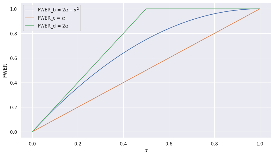
Note: I clipped the function obtained from (d) as the extreme assumption breaks down at \(\alpha = 0.5\)

Q2.

(a)

If we model the rejection of the \(j\text{th}\) null hypothesis as a success, then the distribution of \(A_{j}\) would be:

\[ A_j \sim \text{Bernoulli}(\alpha) \]

(b)

The sum of the \(m\) Bernoulli trials would be Binomial with parameters \(m\) and \(\alpha\):

\[ \sum^m_{j=1} A_j \sim B(m, \alpha) \]

(c) The standard deviation of a Binomial distribution with parameters \(m\) and \(\alpha\) would be:

\[ \sqrt{m \alpha (1 - \alpha)} \]

Q3.

To argue that:

\[ \text{FWER}(\alpha) \le \sum^m_{j = 1} \alpha_j \]

We’ll start with the defintion of the \(\text{FWER}\) and make the assumptions that the \(m\) tests are independent and all the \(m\) null hypotheses are true:

\[\begin{align*} \text{FWER}(\alpha) &= \text{Pr} \left( V \ge 1 \right) \\ &= \text{Pr} \left( \text{falsely reject at least one null hypothesis} \right) \\ &= \text{Pr} \left( \bigcup^m_{j = 1} \{ \text{reject} \space H_{0j} \} \right) \\ &\le \sum^m_{j = 1} \text{Pr} \left( \{ \text{reject} \space H_{0j} \} \right) \\ &\le \sum^m_{j = 1} \alpha_j \\ \end{align*}\]

Where the inequality results from the fact that for any two events \(A\) and \(B\), \(\text{Pr}(A \cup B) \le \text{Pr}(A) + \text{Pr}(B)\).

Q4.

(a) We would reject the null hypotheses for values of \(p\) less than \(0.05\) namely:

\[ H_{01}, H_{02}, H_{03}, H_{08}, H_{09}, H_{10} \]

(b) We would reject the null hypotheses for values of \(p\) less than \(0.005\) which is an \(\alpha\) adjusted for multiple testing (\(\alpha/m\)), which are the following:

\[ H_{01}, H_{09}, H_{10} \]

(c) When controlling the \(\text{FDR}\) at level \(q = 0.05\),

ps = np.array([0.0011, 0.031, 0.017,0.32, 0.11, 0.90, 0.07, 0.006,  0.004, 0.0009])
q = 0.05
fdr05 = multipletests(ps, alpha=q, method="fdr_bh")[0]
np.arange(1, 11)[fdr05]

array([ 1,  3,  8,  9, 10])

We would reject the following null hyoptheses:

\[ H_{01}, H_{03}, H_{08}, H_{09}, H_{10} \]

(d) And when controlling it at level \(q = 0.2\),

ps = np.array([0.0011, 0.031, 0.017,0.32, 0.11, 0.90, 0.07, 0.006,  0.004, 0.0009])
q = 0.2
fdr05 = multipletests(ps, alpha=q, method="fdr_bh")[0]
np.arange(1, 11)[fdr05]

array([ 1,  2,  3,  5,  7,  8,  9, 10])

We would reject the following null hyoptheses:

\[ H_{01}, H_{02}, H_{03}, H_{05}, H_{07}, H_{08}, H_{09}, H_{10} \]

(e) Out of the \(8\) rejected null hypotheses no more than \(20\%\) or approximately \(2\) of them are false positives, because by definition that’s what controlling the \(\text{FDR}\) at level \(20\%\) means.

Q5.

(a)

I can simply pick one \(p\)-value which would get rejected by Bonferroni (\(\le 0.1/5\)), which guarantees being rejected by Holm, then pick \(4\) others that are too big to even consider rejecting.

\[ p_1 = 0.01 \qquad p_2 = 0.5 \qquad p_3 = 0.8 \]

\[ p_4 = 0.2 \qquad p_5 = 0.4 \]

And we’ll verify that both methods reject \(1\) null hypothesis like so:

ps = [0.01, 0.5, 0.8, 0.2, 0.4]
alpha = 0.1

bonf_rejected = multipletests(ps, method="bonf", alpha=alpha)[0].sum()
holm_rejected = multipletests(ps, method="holm", alpha=alpha)[0].sum()

print(f"Rejected by Bonferroni's method: {bonf_rejected}")
print(f"Rejected by Holm's method: {holm_rejected}")

Rejected by Bonferroni's method: 1
Rejected by Holm's method: 1

(b)

For this part I’m going to pick one value to be less than the Bonferroni threshold \(\alpha/m = 0.1/5 = 0.02\) and two values very slightly above that threshold so they get rejected by holm.

\[ p_1 = 0.02 \qquad p_2 = 0.5 \qquad p_3 = 0.1 \]

\[ p_4 = 0.025 \qquad p_5 = 0.03 \]

Verifying that our \(p\)-values satisfy the requirements:

ps = [0.02, 0.5, 0.1, 0.025, 0.03]
alpha = 0.1

bonf_rejected = multipletests(ps, method="bonf", alpha=alpha)[0].sum()
holm_rejected = multipletests(ps, method="holm", alpha=alpha)[0].sum()

print(f"Rejected by Bonferroni's method: {bonf_rejected}")
print(f"Rejected by Holm's method: {holm_rejected}")

Rejected by Bonferroni's method: 1
Rejected by Holm's method: 3

Q6.

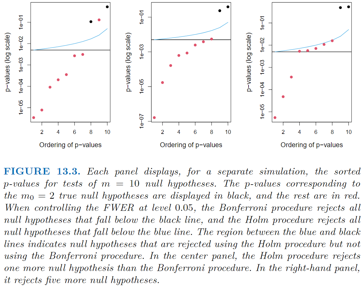
(a) Applying the Bonferroni procedure to control the FWER at level \(\alpha = 0.05\)

Panel 1:

true postives = \(7\)
true negatives = \(2\)
false positives = Type \(\text{I}\) errors = \(0\)
false negatives = Type \(\text{II}\) errors = \(1\)

Panel 2:

true postives = \(7\)
true negatives = \(2\)
false positives = Type \(\text{I}\) errors = \(0\)
false negatives = Type \(\text{II}\) errors = \(1\)

Panel 3:

true postives = \(3\)
true negatives = \(2\)
false positives = Type \(\text{I}\) errors = \(0\)
false negatives = Type \(\text{II}\) errors = \(5\)

(b) Applying the Holm procedure to control the FWER at level \(\alpha = 0.05\)

Panel 1:

true postives = \(7\)
true negatives = \(2\)
false positives = Type \(\text{I}\) errors = \(0\)
false negatives = Type \(\text{II}\) errors = \(1\)

Panel 2:

true postives = \(8\)
true negatives = \(2\)
false positives = Type \(\text{I}\) errors = \(0\)
false negatives = Type \(\text{II}\) errors = \(0\)

Panel 3:

true postives = \(8\)
true negatives = \(2\)
false positives = Type \(\text{I}\) errors = \(0\)
false negatives = Type \(\text{II}\) errors = \(0\)

(c) The false discovery proportion or \(\text{FDP}\) equals \(V/R\) where \(V\) is the number of false positives and \(R\) is total number of rejected null hypotheses which equals the number of true positives + false positives:

Since \(V = 0\) for all three panels then the \(\text{FDP} = 0\) for all three panels.

\[ \text{FDP} = \frac{V}{R} = 0 \]

(d) The same applies here.

\[ \text{FDP} = \frac{V}{R} = 0 \]

(e) Answering (a) and (c) but applying the Bonferroni procedure to control the \(\text{FWER}\) at level \(\alpha = 0.001\) instead, this means rejecting all null hypotheses with \(p\)-values below a horizontal line drawn at \(0.001/10 = 0.0001\)

Panel 1:

true postives = \(3\)
true negatives = \(2\)
false positives = Type \(\text{I}\) errors = \(0\)
false negatives = Type \(\text{II}\) errors = \(5\)

Panel 2:

true postives = \(2\)
true negatives = \(2\)
false positives = Type \(\text{I}\) errors = \(0\)
false negatives = Type \(\text{II}\) errors = \(6\)

Panel 3:

true postives = \(2\)
true negatives = \(2\)
false positives = Type \(\text{I}\) errors = \(0\)
false negatives = Type \(\text{II}\) errors = \(6\)

The \(\text{FDP}\) would again be equal to \(0\) in all three panels since \(V = 0\).

Applied

Q7.

carseats = load_data("Carseats")
carseats.head()

	Sales	CompPrice	Income	Advertising	Population	Price	ShelveLoc	Age	Education	Urban	US
0	9.50	138	73	11	276	120	Bad	42	17	Yes	Yes
1	11.22	111	48	16	260	83	Good	65	10	Yes	Yes
2	10.06	113	35	10	269	80	Medium	59	12	Yes	Yes
3	7.40	117	100	4	466	97	Medium	55	14	Yes	Yes
4	4.15	141	64	3	340	128	Bad	38	13	Yes	No

(a)

numerical_cols = carseats.select_dtypes("number").columns.drop("Sales")
numerical_cols

Index(['CompPrice', 'Income', 'Advertising', 'Population', 'Price', 'Age',
       'Education'],
      dtype='object')

y = carseats["Sales"]
y.shape

(400,)

Now fitting the models for each of the numerical columns on Sales and reporting the \(p\)-value associated with the coefficients:

pvals = dict()
for col in numerical_cols:
    X = sm.add_constant(carseats[col])
    ols = sm.OLS(y, X).fit()
    pval = ols.pvalues.iloc[1]
    pvals[col] = pval

pval_df = pd.DataFrame.from_dict(pvals, orient='index', columns=['p_value'])
pval_df

	p_value
CompPrice	2.009398e-01
Income	2.309670e-03
Advertising	4.377677e-08
Population	3.139816e-01
Price	7.618187e-21
Age	2.788950e-06
Education	2.999442e-01

(b)

pval_df[pval_df["p_value"] < 0.05]

	p_value
Income	2.309670e-03
Advertising	4.377677e-08
Price	7.618187e-21
Age	2.788950e-06

We reject the null hypotheses \(\beta_1 = 0\) associated with \(p\)-values \(\le 0.05\), which are the following variables Income, Advertising, Price, Age.

(c) To control the \(\text{FWER}\) at level \(0.05\), that means we have to reject all null hypotheses with \(p\)-values less than \(0.05/m\), where \(m\) is the number of hypotheses which equals \(7\) here.

len(pval_df)

7

pval_df[pval_df["p_value"] < 0.05/len(pval_df)]

	p_value
Income	2.309670e-03
Advertising	4.377677e-08
Price	7.618187e-21
Age	2.788950e-06

Again we reject the null hypothesis \(\beta_1 = 0\) for all these variables Income, Advertising, Price, Age.

(d) Controlling the \(\text{FDR}\) at level \(0.2\)

fdr20 = multipletests(pval_df["p_value"], method="fdr_bh", alpha=0.2)[0]
pval_df[fdr20]

	p_value
Income	2.309670e-03
Advertising	4.377677e-08
Price	7.618187e-21
Age	2.788950e-06

And again we reject the null hypotheses for all these variables Income, Advertising, Price, Age.

Q8.

rng = np.random.default_rng(1)
n, m = 20, 100
X = rng.normal(size=(n, m))

(a)

pvals = dict()
for i in range(X.shape[1]):
    pvals[i] = ttest_1samp(X[:,i], popmean=0.0).pvalue
    
pval_df = pd.DataFrame.from_dict(pvals, orient='index', columns=['p_value'])
pval_df.head()

	p_value
0	0.053880
1	0.202573
2	0.856777
3	0.619587
4	0.466054

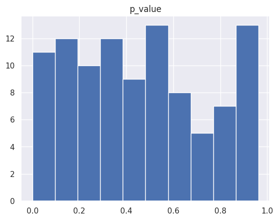
pval_df.hist();

(b)

pval_df[pval_df["p_value"] < 0.05]

	p_value
14	0.000807
27	0.035539
39	0.022933
44	0.009551

We reject \(4\) null hypotheses at level \(\alpha = 0.05\)

(c)

multipletests(pval_df["p_value"], alpha=0.05, method="bonferroni")[0].sum()

0

We fail to reject any null hypotheses when controlling the \(\text{FWER}\) at level \(0.05\).

(d)

multipletests(pval_df["p_value"], alpha=0.05, method="fdr_bh")[0].sum()

0

Again we fail to reject any when controlling the \(\text{FDR}\) at level \(0.05\).

(e) We’ll start by picking the \(10\) fund managers who perform the best in our data.

top10 = pval_df.sort_values(by="p_value")[:10]
top10

	p_value
14	0.000807
44	0.009551
39	0.022933
27	0.035539
72	0.050266
0	0.053880
50	0.065646
20	0.075501
9	0.077960
35	0.087938

Controlling the \(\text{FWER}\) at level \(0.05\)

multipletests(top10["p_value"], alpha=0.05, method="holm")[0].sum()

1

We reject \(1\) null hypothesis.

Now controlling the \(\text{FDR}\) at level \(0.05\)

multipletests(top10["p_value"], alpha=0.05, method="fdr_bh")[0].sum()

2

We reject \(2\) null hypotheses here.

(f) The analysis in (e) is misleading because when we “cherry-pick” the smallest \(p\)-values it’s the same as if we performed \(1000\) tests implicitly, but without adjusting for multiple testing, which results in us rejecting null hypotheses that we wouldn’t reject had we adjusted for multiple testing, purely due to chance.