Ch3: Linear Regression

import numpy as np
import pandas as pd
import matplotlib.pyplot as plt
import seaborn as sns
import statsmodels.api as sm

from statsmodels.stats.anova import anova_lm
from ISLP.models import summarize, poly
from ISLP.models import ModelSpec as MS
from ISLP import load_data

%matplotlib inline

Conceptual

Q1.

The p-values in table 3.4 correspond to null hypotheses where their respective coeffecient equals 0.

\[\begin{split} \begin{aligned} \beta_{intercept} = 0 \\ \beta_{TV} = 0 \\ \beta_{radio} = 0 \\ \beta_{newspaper} = 0 \end{aligned} \end{split}\]

From the p-value results in that table we can reject the null hypothesis for the intercept,TV,radio because of their very small p-values, however we fail to reject the null hypothesis for the newspaper because of its big p-value.

Q2.

The KNN classifier predicts the class of a given value based on the k nearest neighbors to that value.

The KNN regression tries to fit a curve using the average of the k nearest neighbors to the point.

Q3.

b0 = 50
b1 = 20 
b2 = 0.07
b3 = 35
b4 = 0.01
b5 = -10

def predict(GPA: float, IQ: int, College: bool):
    return b0 + b1 * GPA + b2 * IQ + b3 * College + b4 * (GPA * IQ) + b5 * (GPA * College)

GPA = np.arange(2, 4.1, 0.1)
IQ = 100
np.nonzero(np.isclose(predict(GPA, IQ, 1), predict(GPA, IQ, 0)) == 1), GPA[15]

((array([15]),), 3.5000000000000013)

np.mean(predict(GPA[15:], IQ, 0))

135.75000000000003

np.mean(predict(GPA[15:], IQ, 1))

133.25

(a) Statements 3 is correct, because high school graduates earn more on average given the GPA is 3.5 or greater. The increase for going to college (35) is negated by the interaction effect of GPA and Level which has a coefficient of -10. At GPA 3.5 they’d be equal and cancel eachother out. As for GPAs less than 3.5 college graduates earn more.

(b) $137.1k

predict(4.0, 110, 1)

137.1

(C) False, because the value of the coefficient isn’t what affects our confidence in the result rather it’s the p-value for that coefficient.

Q4.

(a) We would expect the \(RSS_{training}\) for the cubic regression to be smaller than that of the linear regression since the cubic would fit closer to the actual points in the dataset. (though this is not a good thing in this case as it’s fitting to the noise in the data (overfitting) while the true relationship is linear)

(b) We would expect the \(RSS_{test}\) for the linear regression to be smaller than the cubic one because the true underlying relationship between X and Y is linear.

(c) We would also expect the training RSS to be smaller for the cubic regression because it’s a more flexible model.

(d) There’s not enough information to tell which test RSS would end up smaller as that depends on how close the underlying relationship is to a linear or a cubic relationship.

Q5.

\[\begin{split} \hat{y_i} = x_i \hat{\beta} \\ \end{split}\]

\[\begin{split} \hat\beta = (\sum_{i=1}^{n} x_i y_i) / (\sum_{i'=1}^{n} x_{i'}^2)\\ \end{split}\]

\[ \hat\beta = \frac{x_1 y_1 + x_2 y_2 + ... + x_n y_n}{x_1^2 + x_2 ^2 + ... + x_n ^2} \]

\[ \hat{y_i} = x_i \frac{x_1 y_1 + x_2 y_2 + ... + x_n y_n}{x_1^2 + x_2 ^2 + ... + x_n ^2} \qquad \text{(1)} \]

\[ \hat{y_i} = \sum_{i'=1}^{n} a_{i'}y_{i'} \]

\[ \hat{y_i} = a_1 y_1 + a_2 y_2 + ... + a_n y_n \qquad \text{(2)} \]

Equating \(\text{(1)}\) and \(\text{(2)}\).

\[ x_i \frac{x_1 y_1 + x_2 y_2 + ... + x_n y_n}{x_1^2 + x_2 ^2 + ... + x_n ^2} = a_1 y_1 + a_2 y_2 + ... + a_n y_n \]

Equating the coefficients of every \(y_{i}\):

\[ a_{i'} = x_i * \frac{x_{i'}}{\sum_{j=1}^{n} x_j^2} \]

Q6.

It’s a simple proof since:

\[ \hat\beta_0 = \bar{y} - \hat\beta_1 \bar{x} \]

Rewriting it:

\[ \bar{y} = \hat\beta_0 + \hat\beta_1 \bar{x} \]

which is the equation for a straight line with intercept \(\hat\beta_0\) and slope \(\hat\beta_1\) and passes through the points \(\bar{y}\) and \(\bar{x}\) and is also the regression line.

Q7.

Given that:

\[ R^2 = \frac{TSS - RSS}{TSS} = 1 - \frac{RSS}{TSS} = 1 - \frac{\sum_{i=1}^{n} (y_i -\hat{y_i})^2}{\sum_{i=1}^{n} (y_i -\bar{y_i})^2} \]

\[ Cor(X, Y) = \frac{\sum_{i=1}^{n} (x_i -\bar{x_i}) (y_i -\bar{y_i})}{\sqrt{\sum_{i=1}^{n} (x_i -\bar{x_i})^2} \sqrt{\sum_{i=1}^{n}(y_i -\bar{y_i})^2}} \]

Prove that:

\[ R^2 = Cor(X, Y)^2 \]

Assuming \(\bar{x} = \bar{y} = 0\) for simplicity

\[ Cor(X, Y) = \frac{\sum_{i=1}^{n} x_i y_i}{\sqrt{\sum_{i=1}^{n} x_i^2} \sqrt{\sum_{i=1}^{n}y_i^2}} \]

Since

\[\begin{split} \bar{x} = \bar{y} = 0 \\ \hat\beta_0 = \bar{y} - \hat\beta_1 \bar{x} \end{split}\]

Then

\[ \hat\beta_0 = 0 \]

and

\[ \hat{y_i} = x_i \frac{\sum_{i=1}^{n} x_i y_i}{\sum_{i'=1}^{n} x_{i'}^2} \]

\[ R^2 = 1 - \frac{\sum_{i=1}^{n} (y_i - x_i \frac{\sum_{i=1}^{n} x_i y_i}{\sum_{i'=1}^{n} x_{i'}^2} )^2}{\sum_{i=1}^{n} y_i^2} \]

Setting \( R^2 = Cor(X, Y)^2 \) and substituting for their values.

\[ \frac{(\sum_{i=1}^{n} x_i y_i)^2}{\sum_{i=1}^{n} x_i^2 \sum_{i=1}^{n}y_i^2} = 1 - \frac{\sum_{i=1}^{n} (y_i - x_i \frac{\sum_{i=1}^{n} x_i y_i}{\sum_{i'=1}^{n} x_{i'}^2} )^2}{\sum_{i=1}^{n} y_i^2} \]

\[ \frac{(\sum_{i=1}^{n} x_i y_i)^2}{\sum_{i=1}^{n} x_i^2 \sum_{i=1}^{n}y_i^2} = \frac{\sum_{i=1}^{n} y_i^2 - \sum_{i=1}^{n} (y_i - x_i \frac{\sum_{i=1}^{n} x_i y_i}{\sum_{i'=1}^{n} x_{i'}^2} )^2}{\sum_{i=1}^{n} y_i^2} \]

\[ \frac{(\sum_{i=1}^{n} x_i y_i)^2}{\sum_{i=1}^{n} x_i^2} = \sum_{i=1}^{n} y_i^2 - \sum_{i=1}^{n} (y_i - x_i \frac{\sum_{j=1}^{n} x_j y_j}{\sum_{i'=1}^{n} x_{i'}^2} )^2 \]

By expanding the squared difference:

\[ \frac{ ( \sum_{i=1}^{n} x_i y_i )^2}{ \sum_{i=1}^{n} x_i^2 } = \sum_{i=1}^{n} y_i^2 - \sum_{i=1}^{n} (y_i^2 - 2 y_i x_i \frac{\sum_{j=1}^{n} x_j y_j}{\sum_{i'=1}^{n} x_{i'}^2} + (x_i \frac{\sum_{j=1}^{n} x_j y_j}{\sum_{i'=1}^{n} x_{i'}^2})^2) \]

\[ \frac{ ( \sum_{i=1}^{n} x_i y_i )^2}{ \sum_{i=1}^{n} x_i^2 } = \sum_{i=1}^{n} ( 2 y_i x_i \frac{\sum_{j=1}^{n} x_j y_j}{\sum_{i'=1}^{n} x_{i'}^2} - (x_i \frac{\sum_{j=1}^{n} x_j y_j}{\sum_{i'=1}^{n} x_{i'}^2})^2) \]

Factoring out \(\frac{\sum_{i=1}^{n} x_i y_i}{\sum_{i=1}^{n} x_i^2}\) from both sides

\[ \sum_{i=1}^{n} x_i y_i = \sum_{i=1}^{n} 2 y_i x_i - x_i^2 \frac{\sum_{j=1}^{n} x_j y_j}{\sum_{i'=1}^{n} x_{i'}^2} \]

Rearranging to make both sides positive:

\[ \sum_{i=1}^{n} x_i^2 \frac{\sum_{j=1}^{n} x_j y_j}{\sum_{i'=1}^{n} x_{i'}^2} = \sum_{i=1}^{n} y_i x_i \]

Simplifying:

\[ \sum_{j=1}^{n} x_j y_j = \sum_{i=1}^{n} y_i x_i \]

We can see that the left handside equals the right handside.

Applied

Q8.

This question involves the use of simple linear regression on the Auto data set.

auto = load_data('Auto')
auto.head()

	mpg	cylinders	displacement	horsepower	weight	acceleration	year	origin
name
chevrolet chevelle malibu	18.0	8	307.0	130	3504	12.0	70	1
buick skylark 320	15.0	8	350.0	165	3693	11.5	70	1
plymouth satellite	18.0	8	318.0	150	3436	11.0	70	1
amc rebel sst	16.0	8	304.0	150	3433	12.0	70	1
ford torino	17.0	8	302.0	140	3449	10.5	70	1

auto.info()

<class 'pandas.core.frame.DataFrame'>
Index: 392 entries, chevrolet chevelle malibu to chevy s-10
Data columns (total 8 columns):
 #   Column        Non-Null Count  Dtype  
---  ------        --------------  -----  
 0   mpg           392 non-null    float64
 1   cylinders     392 non-null    int64  
 2   displacement  392 non-null    float64
 3   horsepower    392 non-null    int64  
 4   weight        392 non-null    int64  
 5   acceleration  392 non-null    float64
 6   year          392 non-null    int64  
 7   origin        392 non-null    int64  
dtypes: float64(3), int64(5)
memory usage: 27.6+ KB

(a) Use the sm.OLS() function to perform a simple linear regression with mpg as the response and horsepower as the predictor. Use the summarize() function to print the results.

horsepower = auto['horsepower']
mpg = auto['mpg']

X = sm.tools.add_constant(horsepower)
X.head()

	const	horsepower
name
chevrolet chevelle malibu	1.0	130
buick skylark 320	1.0	165
plymouth satellite	1.0	150
amc rebel sst	1.0	150
ford torino	1.0	140

Where const is the intercept

y = mpg

model = sm.OLS(y, X)
results1 = model.fit()
summarize(results1)

	coef	std err	t	P>|t|
const	39.9359	0.717	55.660	0.0
horsepower	-0.1578	0.006	-24.489	0.0

results1.summary()

OLS Regression Results

Dep. Variable:	mpg	R-squared:	0.606
Model:	OLS	Adj. R-squared:	0.605
Method:	Least Squares	F-statistic:	599.7
Date:	Fri, 15 Aug 2025	Prob (F-statistic):	7.03e-81
Time:	21:09:40	Log-Likelihood:	-1178.7
No. Observations:	392	AIC:	2361.
Df Residuals:	390	BIC:	2369.
Df Model:	1
Covariance Type:	nonrobust

	coef	std err	t	P>|t|	[0.025	0.975]
const	39.9359	0.717	55.660	0.000	38.525	41.347
horsepower	-0.1578	0.006	-24.489	0.000	-0.171	-0.145

Omnibus:	16.432	Durbin-Watson:	0.920
Prob(Omnibus):	0.000	Jarque-Bera (JB):	17.305
Skew:	0.492	Prob(JB):	0.000175
Kurtosis:	3.299	Cond. No.	322.

Notes:
[1] Standard Errors assume that the covariance matrix of the errors is correctly specified.

i. Is there a relationship between the predictor and the response?

Yes.

ii. How strong is the relationship between the predictor and the response?

\( R^2 = 0.605 \) So about 60% of the variance in mpg is explained by horsepower.

iii. Is the relationship between the predictor and the response positive or negative?

Negative

iv. What is the predicted mpg associated with a horsepower of 98? What are the associated 95 % confidence and prediction intervals?

prediction = results1.get_prediction(pd.DataFrame({'const': [1.0], 'horsepower':[98]}))
prediction.predicted_mean

array([24.46707715])

95% Confidence Interval:

prediction.conf_int(alpha=0.05)

array([[23.97307896, 24.96107534]])

95% Prediction Interval:

prediction.conf_int(alpha=0.05, obs=True)

array([[14.80939607, 34.12475823]])

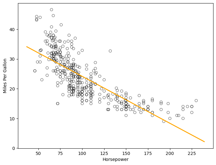
(b) Plot the response and the predictor in a new set of axes ax. Use the ax.axline() method or the abline() function defined in the lab to display the least squares regression line.

_, axes = plt.subplots(figsize=(8,6))
axes.scatter(horsepower, auto['mpg'], marker='o', facecolors='none', edgecolors='black', linewidths=0.5)
axes.set_xlabel('Horsepower')
axes.set_ylabel('Miles Per Gallon')

intercept, slope = results1.params
xlim = axes.get_xlim()
ylim = [intercept + xlim[0] * slope, intercept + xlim[1] * slope]
axes.plot(xlim, ylim, linewidth=2, color='orange');

(c) Produce some of diagnostic plots of the least squares regression fit as described in the lab. Comment on any problems you see with the fit.

with plt.style.context('seaborn-v0_8-darkgrid'):
    _, ax = plt.subplots(figsize=(8,6))
    ax = sns.residplot(x=results1.fittedvalues,y=y,
                            lowess=True,
                            scatter_kws={'alpha': 0.5},
                            line_kws={'color': 'red', 'lw': 1, 'alpha': 0.8})
    ax.set_xlabel('Fitted Values')
    ax.set_ylabel('Residuals')

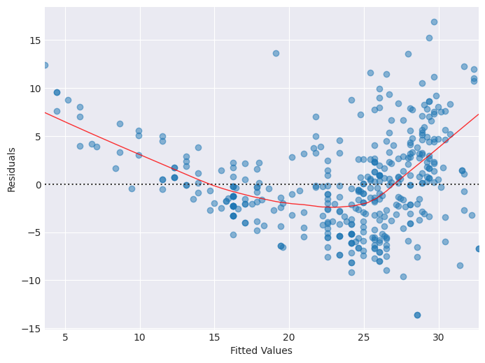
There’s a clear U-shape in the residuals plot indicating the true underlying relationship isn’t linear.

infl = results1.get_influence()
_, ax = plt.subplots(figsize=(8,6))
ax.scatter(np.arange(X.shape[0]), infl.hat_matrix_diag,  marker='o', facecolors='none', edgecolors='black', linewidths=0.5)
ax.set_xlabel('Index')
ax.set_ylabel('Leverage')
np.argmax(infl.hat_matrix_diag)

115

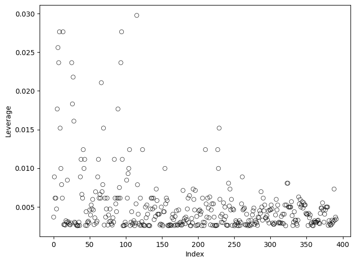
There seems to be a few high leverage points in the data too though we would have to check whether these points have an unusually high leverage.

Q9.

This question involves the use of multiple linear regression on the Auto data set.

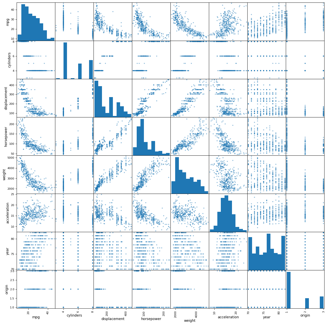
(a) Produce a scatterplot matrix which includes all of the variables in the data set.

pd.plotting.scatter_matrix(auto, figsize=(16, 16));

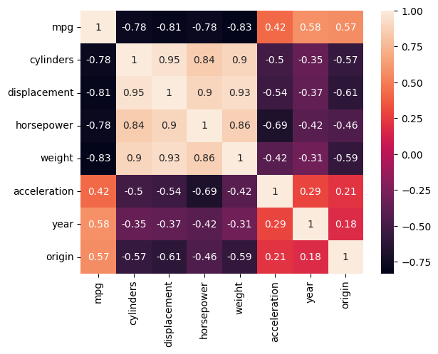
(b) Compute the matrix of correlations between the variables using the DataFrame.corr() method.

sns.heatmap(auto.corr(), annot=True);

(c) Use the sm.OLS() function to perform a multiple linear regression with mpg as the response and all other variables except name as the predictors. Use the summarize() function to print the results. Comment on the output. For instance:

X = auto[auto.columns.drop(['mpg'])]
X.head()

	cylinders	displacement	horsepower	weight	acceleration	year	origin
name
chevrolet chevelle malibu	8	307.0	130	3504	12.0	70	1
buick skylark 320	8	350.0	165	3693	11.5	70	1
plymouth satellite	8	318.0	150	3436	11.0	70	1
amc rebel sst	8	304.0	150	3433	12.0	70	1
ford torino	8	302.0	140	3449	10.5	70	1

y = mpg

X = sm.tools.add_constant(X)
model = sm.OLS(y, X)
results2 = model.fit()
summarize(results2)

	coef	std err	t	P>|t|
const	-17.2184	4.644	-3.707	0.000
cylinders	-0.4934	0.323	-1.526	0.128
displacement	0.0199	0.008	2.647	0.008
horsepower	-0.0170	0.014	-1.230	0.220
weight	-0.0065	0.001	-9.929	0.000
acceleration	0.0806	0.099	0.815	0.415
year	0.7508	0.051	14.729	0.000
origin	1.4261	0.278	5.127	0.000

i. Is there a relationship between the predictors and the response? Use the anova_lm() function from statsmodels to answer this question.

anova_lm(results1, results2)

	df_resid	ssr	df_diff	ss_diff	F	Pr(>F)
0	390.0	9385.915872	0.0	NaN	NaN	NaN
1	384.0	4252.212530	6.0	5133.703341	77.267308	5.376746e-63

Yes there’s strong evidence that there’s a relationship between the predictors and the response.

ii. Which predictors appear to have a statistically significant relationship to the response?

displacement, weight, year, origin all have a statistically significant relationship to the response.

iii. What does the coefficient for the year variable suggest?

It suggests that a one year increase in car production year tends to result in a 0.75 unit increase in mpg.

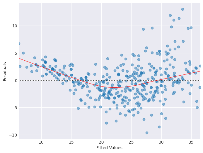
(d) Produce some of diagnostic plots of the linear regression fit as described in the lab. Comment on any problems you see with the fit. Do the residual plots suggest any unusually large outliers? Does the leverage plot identify any observations with unusually high leverage?

with plt.style.context('seaborn-v0_8-darkgrid'):
    _, ax = plt.subplots(figsize=(8,6))
    ax = sns.residplot(x=results2.fittedvalues,y=y,
                            lowess=True,
                            scatter_kws={'alpha': 0.5},
                            line_kws={'color': 'red', 'lw': 1, 'alpha': 0.8})
    ax.set_xlabel('Fitted Values')
    ax.set_ylabel('Residuals')

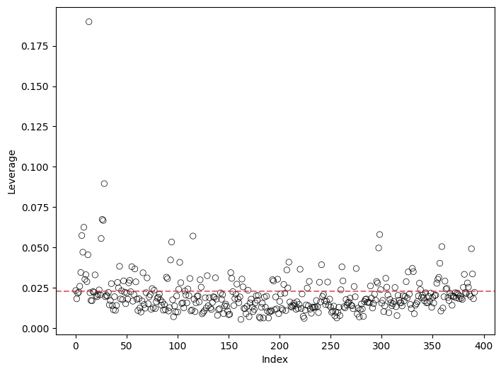
h_avg = ((X.shape[1]+1)/X.shape[0])
h_avg

0.02295918367346939

infl = results2.get_influence()
_, ax = plt.subplots(figsize=(8,6))
ax.scatter(np.arange(X.shape[0]), infl.hat_matrix_diag,  marker='o', facecolors='none', edgecolors='black', linewidths=0.5)
ax.axhline(h_avg, ls='--', c='r', alpha=0.6)
ax.set_xlabel('Index')
ax.set_ylabel('Leverage')
np.argmax(infl.hat_matrix_diag)

13

X.iloc[13]

const              1.0
cylinders          8.0
displacement     455.0
horsepower       225.0
weight          3086.0
acceleration      10.0
year              70.0
origin             1.0
Name: buick estate wagon (sw), dtype: float64

np.arange(X.shape[0])[infl.hat_matrix_diag/h_avg > 3]

array([13, 28])

Points 13 and 28 have a leverage that’s more than 3 times the average leverage.

From the residuals plot we can see that the U-shape persists indicating that the true underlying relationship between the predictors and the response isn’t linear.

We can also see a few large residuals but they’re not unusual due to the difference between the true underlying relationship and the used model.

In the leverage plot we can identify a point with an extremely high leverage that the model would benefit from removing. (the point at index 13)

(e) Fit some models with interactions as described in the lab. Do any interactions appear to be statistically significant?

auto.columns

Index(['mpg', 'cylinders', 'displacement', 'horsepower', 'weight',
       'acceleration', 'year', 'origin'],
      dtype='object')

y = mpg
X = MS(['cylinders', 'horsepower',
        ('cylinders', 'horsepower')]).fit_transform(auto)
model3 = sm.OLS(y, X)
results3 = model3.fit()
summarize(results3)

	coef	std err	t	P>|t|
intercept	72.8151	3.071	23.708	0.0
cylinders	-6.4925	0.511	-12.716	0.0
horsepower	-0.4160	0.035	-12.051	0.0
cylinders:horsepower	0.0472	0.005	9.984	0.0

The relationship between cylinders and horsepower seems to be statistically significant.

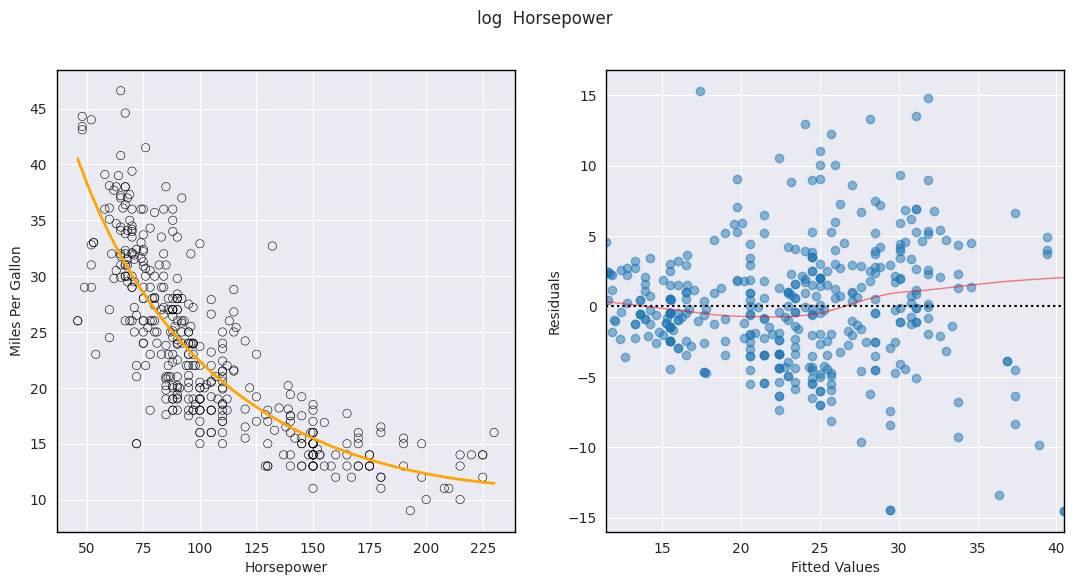
(f) Try a few different transformations of the variables, such as \(\log(X), \sqrt{X}, X^2\). Comment on your findings.

def test_with_transformation(func_list):
    with sns.axes_style("darkgrid") :
        y = mpg
        X = pd.DataFrame({'horsepower': horsepower})
        
        for func in func_list:
            X[f'{func.__name__} horsepower'] = func(horsepower)
        X = sm.tools.add_constant(X)
        results_tests = sm.OLS(y, X).fit()

        fig, axes = plt.subplots(1, 2, figsize=(13, 6))
        
        full_name = ""
        for func in func_list:
            full_name += f'{func.__name__} '
        fig.suptitle(f'{full_name} Horsepower')
        
        axes[0].scatter(horsepower, mpg, marker='o', facecolors='none', edgecolors='black', linewidths=0.4)
        axes[0].set_xlabel('Horsepower')
        axes[0].set_ylabel('Miles Per Gallon')

        xlim = np.sort(horsepower)[0], np.sort(horsepower)[-1]
        x_pred = np.linspace(xlim[0], xlim[1], 500)
        X_pred = pd.DataFrame({'horsepower':x_pred})
        for func in func_list:
            X_pred[f'{func.__name__} horsepower'] = func(x_pred)
        X_pred = sm.tools.add_constant(X_pred)
        y_pred = results_tests.predict(X_pred)
        
        axes[0].plot(x_pred, y_pred, linewidth=2, color='orange');

        sns.residplot(x=results_tests.fittedvalues, y=y,
                    lowess=True,
                    scatter_kws={'alpha': 0.5},
                    line_kws={'color': 'red', 'lw': 1, 'alpha': 0.5},
                    ax=axes[1])
        axes[1].set_xlabel('Fitted Values')
        axes[1].set_ylabel('Residuals')
        axes[1].axhline(0, ls=':', color='k');
        
        for ax in axes: 
            for spine in ax.spines.values():
                spine.set_visible(True)
                spine.set_linewidth(1)
                spine.set_color('black');
        
        return results_tests.summary()

test_with_transformation([np.log])

OLS Regression Results

Dep. Variable:	mpg	R-squared:	0.682
Model:	OLS	Adj. R-squared:	0.680
Method:	Least Squares	F-statistic:	416.6
Date:	Fri, 15 Aug 2025	Prob (F-statistic):	1.98e-97
Time:	21:09:44	Log-Likelihood:	-1136.8
No. Observations:	392	AIC:	2280.
Df Residuals:	389	BIC:	2292.
Df Model:	2
Covariance Type:	nonrobust

	coef	std err	t	P>|t|	[0.025	0.975]
const	156.0406	12.083	12.914	0.000	132.285	179.796
horsepower	0.1185	0.029	4.044	0.000	0.061	0.176
log horsepower	-31.5982	3.284	-9.623	0.000	-38.054	-25.142

Omnibus:	17.484	Durbin-Watson:	1.115
Prob(Omnibus):	0.000	Jarque-Bera (JB):	39.245
Skew:	0.162	Prob(JB):	3.01e-09
Kurtosis:	4.516	Cond. No.	6.26e+03

Notes:
[1] Standard Errors assume that the covariance matrix of the errors is correctly specified.
[2] The condition number is large, 6.26e+03. This might indicate that there are
strong multicollinearity or other numerical problems.

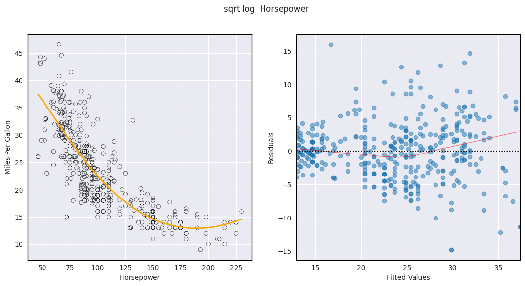
test_with_transformation([np.sqrt, np.log])

OLS Regression Results

Dep. Variable:	mpg	R-squared:	0.690
Model:	OLS	Adj. R-squared:	0.687
Method:	Least Squares	F-statistic:	287.3
Date:	Fri, 15 Aug 2025	Prob (F-statistic):	3.52e-98
Time:	21:09:45	Log-Likelihood:	-1131.9
No. Observations:	392	AIC:	2272.
Df Residuals:	388	BIC:	2288.
Df Model:	3
Covariance Type:	nonrobust

	coef	std err	t	P>|t|	[0.025	0.975]
const	-63.8198	70.990	-0.899	0.369	-203.393	75.754
horsepower	1.3467	0.392	3.435	0.001	0.576	2.117
sqrt horsepower	-51.8974	16.518	-3.142	0.002	-84.373	-19.421
log horsepower	102.1959	42.708	2.393	0.017	18.228	186.164

Omnibus:	16.657	Durbin-Watson:	1.080
Prob(Omnibus):	0.000	Jarque-Bera (JB):	31.290
Skew:	0.233	Prob(JB):	1.60e-07
Kurtosis:	4.303	Cond. No.	4.28e+04

Notes:
[1] Standard Errors assume that the covariance matrix of the errors is correctly specified.
[2] The condition number is large, 4.28e+04. This might indicate that there are
strong multicollinearity or other numerical problems.

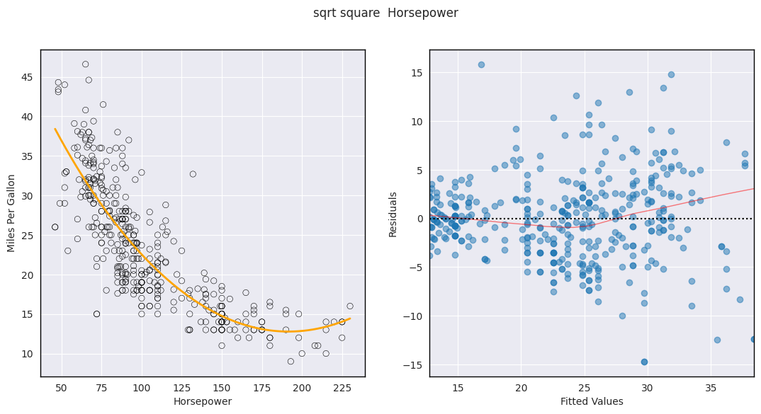
test_with_transformation([np.sqrt, np.square])

OLS Regression Results

Dep. Variable:	mpg	R-squared:	0.688
Model:	OLS	Adj. R-squared:	0.685
Method:	Least Squares	F-statistic:	284.8
Date:	Fri, 15 Aug 2025	Prob (F-statistic):	1.18e-97
Time:	21:09:45	Log-Likelihood:	-1133.1
No. Observations:	392	AIC:	2274.
Df Residuals:	388	BIC:	2290.
Df Model:	3
Covariance Type:	nonrobust

	coef	std err	t	P>|t|	[0.025	0.975]
const	65.3559	23.054	2.835	0.005	20.029	110.682
horsepower	-0.3157	0.410	-0.770	0.442	-1.122	0.491
sqrt horsepower	-2.1514	5.848	-0.368	0.713	-13.649	9.346
square horsepower	0.0010	0.001	1.810	0.071	-8.87e-05	0.002

Omnibus:	16.449	Durbin-Watson:	1.085
Prob(Omnibus):	0.000	Jarque-Bera (JB):	32.200
Skew:	0.210	Prob(JB):	1.02e-07
Kurtosis:	4.340	Cond. No.	1.70e+06

Notes:
[1] Standard Errors assume that the covariance matrix of the errors is correctly specified.
[2] The condition number is large, 1.7e+06. This might indicate that there are
strong multicollinearity or other numerical problems.

test_with_transformation([np.square, np.sqrt, np.log])

OLS Regression Results

Dep. Variable:	mpg	R-squared:	0.695
Model:	OLS	Adj. R-squared:	0.692
Method:	Least Squares	F-statistic:	220.6
Date:	Fri, 15 Aug 2025	Prob (F-statistic):	1.99e-98
Time:	21:09:45	Log-Likelihood:	-1128.3
No. Observations:	392	AIC:	2267.
Df Residuals:	387	BIC:	2287.
Df Model:	4
Covariance Type:	nonrobust

	coef	std err	t	P>|t|	[0.025	0.975]
const	-683.8915	243.904	-2.804	0.005	-1163.435	-204.348
horsepower	11.6464	3.898	2.988	0.003	3.982	19.311
square horsepower	-0.0074	0.003	-2.655	0.008	-0.013	-0.002
sqrt horsepower	-338.4598	109.153	-3.101	0.002	-553.067	-123.852
log horsepower	651.4691	211.145	3.085	0.002	236.334	1066.605

Omnibus:	20.312	Durbin-Watson:	1.103
Prob(Omnibus):	0.000	Jarque-Bera (JB):	38.388
Skew:	0.302	Prob(JB):	4.62e-09
Kurtosis:	4.409	Cond. No.	2.46e+07

Notes:
[1] Standard Errors assume that the covariance matrix of the errors is correctly specified.
[2] The condition number is large, 2.46e+07. This might indicate that there are
strong multicollinearity or other numerical problems.

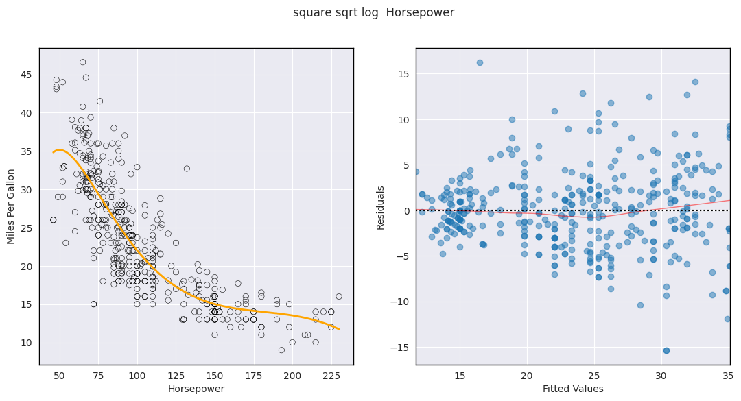
We can see that adding the log term slightly bettered the fit of the model to the data capturing the underlying non-linear relationship a bit better. As we added more terms the U-shape in the residuals plot diminished but heteroscedasticity remained very visible.

The last model with the 3 functions combined seems to be the best fit to the data with the highest \(R^2\) value of 0.695 and we can reject the null hypotheses for all coefficients with a 0.01 confidence level meaning that there’s very likely a relationship between the response and the predictors when they’re together (log sqrt square transformations of horsepower).

Q10.

This question should be answered using the Carseats data set.

carseats = load_data('Carseats')
carseats.head() 

	Sales	CompPrice	Income	Advertising	Population	Price	ShelveLoc	Age	Education	Urban	US
0	9.50	138	73	11	276	120	Bad	42	17	Yes	Yes
1	11.22	111	48	16	260	83	Good	65	10	Yes	Yes
2	10.06	113	35	10	269	80	Medium	59	12	Yes	Yes
3	7.40	117	100	4	466	97	Medium	55	14	Yes	Yes
4	4.15	141	64	3	340	128	Bad	38	13	Yes	No

carseats.info()

<class 'pandas.core.frame.DataFrame'>
RangeIndex: 400 entries, 0 to 399
Data columns (total 11 columns):
 #   Column       Non-Null Count  Dtype   
---  ------       --------------  -----   
 0   Sales        400 non-null    float64 
 1   CompPrice    400 non-null    int64   
 2   Income       400 non-null    int64   
 3   Advertising  400 non-null    int64   
 4   Population   400 non-null    int64   
 5   Price        400 non-null    int64   
 6   ShelveLoc    400 non-null    category
 7   Age          400 non-null    int64   
 8   Education    400 non-null    int64   
 9   Urban        400 non-null    category
 10  US           400 non-null    category
dtypes: category(3), float64(1), int64(7)
memory usage: 26.7 KB

(a) Fit a multiple regression model to predict Sales using Price, Urban, and US.

y = carseats['Sales']
X = MS(['Price', 'Urban', 'US']).fit_transform(carseats)
results = sm.OLS(y, X).fit()
summarize(results)

	coef	std err	t	P>|t|
intercept	13.0435	0.651	20.036	0.000
Price	-0.0545	0.005	-10.389	0.000
Urban[Yes]	-0.0219	0.272	-0.081	0.936
US[Yes]	1.2006	0.259	4.635	0.000

(b) Provide an interpretation of each coefficient in the model. Be careful—some of the variables in the model are qualitative!

Price: for every unit increase in Price the Sales decreases by -0.0545 (sales here are in thousands so that would be 55 sales less).

Urban[Yes]: A dummy variable for the qualitative predictor Urban, tells us that a Store in an urban area has -0.0219 less Sales though it’s not statistically significant.

US[Yes]: A dummy variable for the qualitative predictor US, tells us that a Store in the US has 1.2006 more Sales.

(c) Write out the model in equation form, being careful to handle the qualitative variables properly.

\[ Sales = 13.0435 - 0.0545 \times Price + 1.2006 \times US - 0.0219 \times Urban \]

\[\begin{split} Sales = \begin{cases} 13.0435 - 0.0545 \times Price + 1.2006 - 0.0219 & \text{If US and Urban} \\ 13.0435 - 0.0545 \times Price - 0.0219 & \text{If not US and Urban} \\ 13.0435 - 0.0545 \times Price + 1.2006 & \text{If US and not Urban} \\ 13.0435 - 0.0545 \times Price & \text{If not US and not Urban} \end{cases} \end{split}\]

(d) For which of the predictors can you reject the null hypothesis \(H_0 : β_j = 0\)?

We can reject the null hypothesis for the intercept, Price and US predictors though we can’t reject it for the Urban predictor since it has a very high p-value of 0.936.

(e) On the basis of your response to the previous question, fit a smaller model that only uses the predictors for which there is evidence of association with the outcome.

We’ll just remove the Urban predictor since there’s no evidence it’s associated with the response.

y = carseats['Sales']
X = MS(['Price', 'US']).fit_transform(carseats)
results_no_urban = sm.OLS(y, X).fit()
summarize(results_no_urban)

	coef	std err	t	P>|t|
intercept	13.0308	0.631	20.652	0.0
Price	-0.0545	0.005	-10.416	0.0
US[Yes]	1.1996	0.258	4.641	0.0

(f) How well do the models in (a) and (e) fit the data?

results.summary()

OLS Regression Results

Dep. Variable:	Sales	R-squared:	0.239
Model:	OLS	Adj. R-squared:	0.234
Method:	Least Squares	F-statistic:	41.52
Date:	Fri, 15 Aug 2025	Prob (F-statistic):	2.39e-23
Time:	21:09:46	Log-Likelihood:	-927.66
No. Observations:	400	AIC:	1863.
Df Residuals:	396	BIC:	1879.
Df Model:	3
Covariance Type:	nonrobust

	coef	std err	t	P>|t|	[0.025	0.975]
intercept	13.0435	0.651	20.036	0.000	11.764	14.323
Price	-0.0545	0.005	-10.389	0.000	-0.065	-0.044
Urban[Yes]	-0.0219	0.272	-0.081	0.936	-0.556	0.512
US[Yes]	1.2006	0.259	4.635	0.000	0.691	1.710

Omnibus:	0.676	Durbin-Watson:	1.912
Prob(Omnibus):	0.713	Jarque-Bera (JB):	0.758
Skew:	0.093	Prob(JB):	0.684
Kurtosis:	2.897	Cond. No.	628.

Notes:
[1] Standard Errors assume that the covariance matrix of the errors is correctly specified.

results_no_urban.summary()

OLS Regression Results

Dep. Variable:	Sales	R-squared:	0.239
Model:	OLS	Adj. R-squared:	0.235
Method:	Least Squares	F-statistic:	62.43
Date:	Fri, 15 Aug 2025	Prob (F-statistic):	2.66e-24
Time:	21:09:46	Log-Likelihood:	-927.66
No. Observations:	400	AIC:	1861.
Df Residuals:	397	BIC:	1873.
Df Model:	2
Covariance Type:	nonrobust

	coef	std err	t	P>|t|	[0.025	0.975]
intercept	13.0308	0.631	20.652	0.000	11.790	14.271
Price	-0.0545	0.005	-10.416	0.000	-0.065	-0.044
US[Yes]	1.1996	0.258	4.641	0.000	0.692	1.708

Omnibus:	0.666	Durbin-Watson:	1.912
Prob(Omnibus):	0.717	Jarque-Bera (JB):	0.749
Skew:	0.092	Prob(JB):	0.688
Kurtosis:	2.895	Cond. No.	607.

Notes:
[1] Standard Errors assume that the covariance matrix of the errors is correctly specified.

anova_lm(results, results_no_urban)

	df_resid	ssr	df_diff	ss_diff	F	Pr(>F)
0	396.0	2420.834671	0.0	NaN	NaN	NaN
1	397.0	2420.874462	-1.0	-0.03979	0.006525	NaN

Both models are approximately the same and neither of them is a great fit to the data with \(R^2\) scores of 0.239 though we can say that model (e) is better since it accomplishes the same task with one less predictor.

(g) Using the model from (e), obtain 95 % confidence intervals for the coefficient(s).

results_no_urban.conf_int(alpha=0.05)

	0	1
intercept	11.79032	14.271265
Price	-0.06476	-0.044195
US[Yes]	0.69152	1.707766

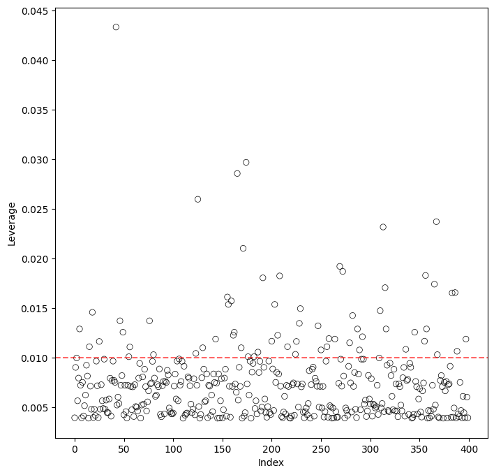
(h) Is there evidence of outliers or high leverage observations in the model from (e)?

h_avg = ((X.shape[1]+1)/X.shape[0])
h_avg

0.01

infl = results_no_urban.get_influence()
_, ax = plt.subplots(figsize=(8,8))
ax.scatter(np.arange(X.shape[0]), infl.hat_matrix_diag, marker='o', facecolors='none', edgecolors='black', linewidths=0.5)
ax.axhline(h_avg, ls='--', c='r', alpha=0.6)
ax.set_xlabel('Index')
ax.set_ylabel('Leverage')
np.argmax(infl.hat_matrix_diag)

42

np.arange(X.shape[0])[infl.hat_matrix_diag/h_avg > 3]

array([42])

infl.hat_matrix_diag[42]/h_avg

4.3337657037178525

The point at index 42 has very high leverage compared to the rest of the data, precisely 4.33 times the average leverage.

X.iloc[42]

intercept     1.0
Price        24.0
US[Yes]       0.0
Name: 42, dtype: float64

X.describe()

	intercept	Price	US[Yes]
count	400.0	400.000000	400.000000
mean	1.0	115.795000	0.645000
std	0.0	23.676664	0.479113
min	1.0	24.000000	0.000000
25%	1.0	100.000000	0.000000
50%	1.0	117.000000	1.000000
75%	1.0	131.000000	1.000000
max	1.0	191.000000	1.000000

It also happens to be the point with the minimum price.

Q11.

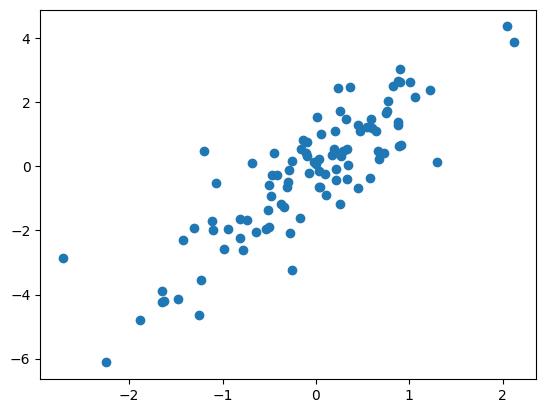
In this problem we will investigate the t-statistic for the null hypoth- esis H0 : β = 0 in simple linear regression without an intercept. To begin, we generate a predictor x and a response y as follows.

rng = np.random.default_rng (1)
x = rng.normal(size =100)
y = 2 * x + rng.normal(size =100)

plt.scatter(x, y);

(a) Perform a simple linear regression of y onto x, without an intercept. Report the coefficient estimate \(\hat\beta\), the standard error of this coefficient estimate, and the t-statistic and p-value associated with the null hypothesis \(H_0 : \beta = 0\). Comment on these results. (You can perform regression without an intercept using the keywords argument intercept=False to ModelSpec().

df = pd.DataFrame({'x': x, 'y':y})
X = MS('x', intercept=False).fit_transform(df)
results = sm.OLS(y, X).fit()
summarize(results)

	coef	std err	t	P>|t|
x	1.9762	0.117	16.898	0.0

The value for the coefficient \(\hat\beta\) we got is pretty close to 2 which is the number we multiplied by x to get y. The relationship between x and y is statistically significant.

(b) Now perform a simple linear regression of x onto y without an intercept, and report the coefficient estimate, its standard error, and the corresponding t-statistic and p-values associated with the null hypothesis \(H_0 : \beta = 0\). Comment on these results.

df = pd.DataFrame({'x': x, 'y':y})
Y = MS('y', intercept=False).fit_transform(df)
results = sm.OLS(x, Y).fit()
summarize(results)

	coef	std err	t	P>|t|
y	0.3757	0.022	16.898	0.0

Naturally there’s a relationship and it’s also statistically significant.

(c) What is the relationship between the results obtained in (a) and (b)?

They have the same exact t-statistic.

And I think they should be reciprocals of eachother but the other regression coefficient was very badly affected by noise which let it get pretty far from 0.5.

This is a better and more naunced answer

https://botlnec.github.io/islp/sols/chapter3/exercise11/#c

(d) Check the book for the full question but the jist of it is:

Given that:

\[\begin{split} \hat\beta = (\sum_{i=1}^{n} x_i y_i) / (\sum_{i'=1}^{n} x_{i'}^2)\\ \end{split}\]

\[ SE(\hat\beta) = \sqrt{\frac{\sum_{i=1}^{n} (y_i - x_i \hat\beta) ^ 2}{(n - 1) \sum_{i'=1}^{n} x_{i'}^2}} \]

Prove that:

\[ \hat\beta / SE(\hat\beta) = \frac{\sqrt{n-1} \sum_{i=1}^{n} x_i y_i}{\sqrt{(\sum_{i=1}^{n} x_i^2) (\sum_{i'=1}^{n} y_{i'}^2) - (\sum_{i'=1}^{n} x_{i'} y_{i'}) ^ 2}} \]

Solution:

Dividing both sides:

\[ \hat\beta / SE(\hat\beta) = \frac{\sqrt{n - 1} \sqrt{\sum_{i'=1}^{n} x_{i'}^2} \sum_{i=1}^{n} x_i y_i}{\sum_{i'=1}^{n} x_{i'}^2 \sqrt{\sum_{i=1}^{n} (y_i - x_i \hat\beta)^2}} \]

Substituting for \(\hat\beta\) and factoring out \(\sqrt{\sum_{i'=1}^{n} x_{i'}^2}\) from the numerator and denominator:

\[ \hat\beta / SE(\hat\beta) = \frac{\sqrt{n - 1} \sum_{i=1}^{n} x_i y_i}{\sqrt{\sum_{i'=1}^{n} x_{i'}^2} \sqrt{\sum_{i=1}^{n} (y_i - x_i \frac{\sum_{j=1}^{n} x_j y_j}{\sum_{i'=1}^{n} x_{i'}^2})^2}} \]

By expanding the squared difference:

\[ \hat\beta / SE(\hat\beta) = \frac{\sqrt{n - 1} \sum_{i=1}^{n} x_i y_i}{\sqrt{\sum_{i'=1}^{n} x_{i'}^2} \sqrt{\sum_{i=1}^{n} (y_i^2 - 2 y_i x_i \frac{\sum_{j=1}^{n} x_j y_j}{\sum_{i'=1}^{n} x_{i'}^2} + (x_i \frac{\sum_{j=1}^{n} x_j y_j}{\sum_{i'=1}^{n} x_{i'}^2})^2) }} \]

And simplifying:

\[ \hat\beta / SE(\hat\beta) = \frac{\sqrt{n - 1} \sum_{i=1}^{n} x_i y_i}{\sqrt{\sum_{i=1}^{n} \sum_{i'=1}^{n} x_{i'}^2 y_i^2 - 2 \sum_{i=1}^{n} y_i x_i \sum_{j=1}^{n} x_j y_j + (\sum_{j=1}^{n} x_j y_j)^2}} \]

\[ \hat\beta / SE(\hat\beta) = \frac{\sqrt{n - 1} \sum_{i=1}^{n} x_i y_i}{\sqrt{\sum_{i=1}^{n} \sum_{i'=1}^{n} x_{i'}^2 y_i^2 - 2 (\sum_{j=1}^{n} x_j y_j)^2 + (\sum_{j=1}^{n} x_j y_j)^2}} \]

\[ \hat\beta / SE(\hat\beta) = \frac{\sqrt{n - 1} \sum_{i=1}^{n} x_i y_i}{\sqrt{(\sum_{i=1}^{n} x_{i'}^2) (\sum_{i'=1}^{n} y_i^2) - (\sum_{j=1}^{n} x_j y_j)^2 }} \]

Which is what we set out to prove.

All that’s left is confirming that the t-statistic can be calculated using that formula numerically.

def t(x, y):
    n = x.shape[0]
    numerator = np.sqrt(n - 1) * np.sum(x * y)
    denominator = np.sqrt(np.sum(x**2) * np.sum(y**2) - (np.sum(x * y))**2)
    return numerator/denominator 

t(x, y), results.tvalues

(16.898417063035094,
 y    16.898417
 dtype: float64)

Which is exactly the same as the value returned from the fitted results summary earlier.

(e) Using the results from (d), argue that the t-statistic for the regression of y onto x is the same as the t-statistic for the regression of x onto y.

Simply substituing x with y and y with x we can see that the formula remains exactly the same.

We can also try that numerically too.

t(y, x)

16.898417063035094

(f) Show that when regression is performed with an intercept, the t-statistic for \(H_0 : \beta_1 = 0\) is the same for the regression of y onto x as it is for the regression of x onto y.

df = pd.DataFrame({'x': x, 'y':y})
X = MS('x').fit_transform(df)
results = sm.OLS(y, X).fit()
summarize(results)

	coef	std err	t	P>|t|
intercept	-0.0760	0.101	-0.756	0.451
x	1.9686	0.118	16.734	0.000

df = pd.DataFrame({'x': x, 'y':y})
Y = MS('y').fit_transform(df)
results = sm.OLS(x, Y).fit()
summarize(results)

	coef	std err	t	P>|t|
intercept	0.0095	0.044	0.216	0.829
y	0.3763	0.022	16.734	0.000

As we can see the t-statistic for \(H_0 : \beta_1 = 0\) is 16.734 for both regressions y onto x and x onto y.

Q12.

This problem involves simple linear regression without an intercept

(a) Recall that the coefficient estimate \(\hat\beta\) for the linear regression of Y onto X without an intercept is given by (3.38). Under what circumstance is the coefficient estimate for the regression of X onto Y the same as the coefficient estimate for the regression of Y onto X?

When they have the same variance or one of them is a permutation of the other.

(b) Generate an example in Python with n = 100 observations in which the coefficient estimate for the regression of X onto Y is different from the coefficient estimate for the regression of Y onto X.

rng = np.random.default_rng(1)
x = rng.normal(size =100)
y = 2 * x + rng.normal(size =100)
plt.scatter(x, y);

df = pd.DataFrame({'x': x, 'y':y})
X = MS('x', intercept=False).fit_transform(df)
results = sm.OLS(y, X).fit()
summarize(results)

	coef	std err	t	P>|t|
x	1.9762	0.117	16.898	0.0

df = pd.DataFrame({'x': x, 'y':y})
Y = MS('y', intercept=False).fit_transform(df)
results = sm.OLS(x, Y).fit()
summarize(results)

	coef	std err	t	P>|t|
y	0.3757	0.022	16.898	0.0

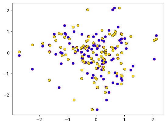
(c) Generate an example in Python with n = 100 observations in which the coefficient estimate for the regression of X onto Y is the same as the coefficient estimate for the regression of Y onto X.

rng = np.random.default_rng(1)
x = rng.normal(size =100)
y = rng.permutation(x)
plt.scatter(x, y,  marker='o', facecolors='blue', edgecolors='red', linewidths=0.5);
plt.scatter(y, x,  marker='o', facecolors='gold', edgecolors='black', linewidths=0.5);

df = pd.DataFrame({'x': x, 'y':y})
X = MS('x', intercept=False).fit_transform(df)
results = sm.OLS(y, X).fit()
summarize(results)

	coef	std err	t	P>|t|
x	-0.0565	0.1	-0.563	0.575

df = pd.DataFrame({'x': x, 'y':y})
Y = MS('y', intercept=False).fit_transform(df)
results = sm.OLS(x, Y).fit()
summarize(results)

	coef	std err	t	P>|t|
y	-0.0565	0.1	-0.563	0.575

Q13.

In this exercise you will create some simulated data and will fit simple linear regression models to it. Make sure to use the default random number generator with seed set to 1 prior to starting part (a) to ensure consistent results.

(a) Using the normal() method of your random number generator, create a vector, x, containing 100 observations drawn from a \(N(0, 1)\) distribution. This represents a feature, X.

rng = np.random.default_rng(1)
x = rng.normal(0, 1, size=100)

(b) Using the normal() method, create a vector, eps, containing 100 observations drawn from a \(N(0, 0.25)\) distribution—a normal distribution with mean zero and variance 0.25.

eps = rng.normal(0, 0.25, size=100)

(c) Using x and eps, generate a vector y according to the model

\[ Y = -1 + 0.5X + \epsilon \]

What is the length of the vector y ? What are the values of \(\beta_0\) and \(\beta_1\) in this linear model?

y = -1 + 0.5 * x + eps
y.shape

(100,)

The length of y is 100. \(\beta_0 = -1\) and \(\beta_1 = 0.5\).

(d) Create a scatterplot displaying the relationship between x and y. Comment on what you observe.

plt.scatter(x, y)
plt.xlabel('x')
plt.ylabel('y');

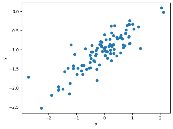
There’s a very obvious linear relationship between x and y. You can also roughly make out the position of the intercept to be at -1.

(e) Fit a least squares linear model to predict y using x. Comment on the model obtained. How do \(\hat\beta_0\) and \(\hat\beta_1\) compare to \(\beta_0\) and \(\beta_1\)?

df = pd.DataFrame({'x': x, 'y':y})
X = MS('x').fit_transform(df)
results = sm.OLS(y, X).fit()
summarize(results)

	coef	std err	t	P>|t|
intercept	-1.0190	0.025	-40.537	0.0
x	0.4921	0.029	16.734	0.0

The predicted coefficients are very close to the true coefficients.

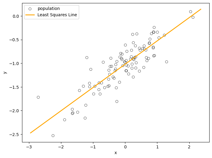
(f) Display the least squares line on the scatterplot obtained in (d). Draw the population regression line on the plot, in a different color. Use the legend() method of the axes to create an appropriate legend

_, ax = plt.subplots(figsize=(8,6))
ax.scatter(x, y, marker='o', facecolors='none', edgecolors='black', linewidths=0.5, label='population')
ax.set_xlabel('x')
ax.set_ylabel('y')

intercept, slope = results.params
xlim = ax.get_xlim()
ylim = [intercept + xlim[0] * slope, intercept + xlim[1] * slope]
ax.plot(xlim, ylim, linewidth=2, color='orange', label='Least Squares Line')
ax.legend();

(g) Now fit a polynomial regression model that predicts y using x and \(x^2\) . Is there evidence that the quadratic term improves the model fit? Explain your answer.

X = MS([poly('x', degree=2)]).fit_transform(df)
results_poly = sm.OLS(y, X).fit()
summarize(results_poly)

	coef	std err	t	P>|t|
intercept	-1.0552	0.025	-41.920	0.000
poly(x, degree=2)[0]	4.1909	0.252	16.649	0.000
poly(x, degree=2)[1]	-0.0131	0.252	-0.052	0.959

We can see that the p-value for the quadratic term is 0.959 which is extremely high, indicating that we cannot reject the null hypothesis here hence we have no reason to believe that the quadratic term improves the model fit.

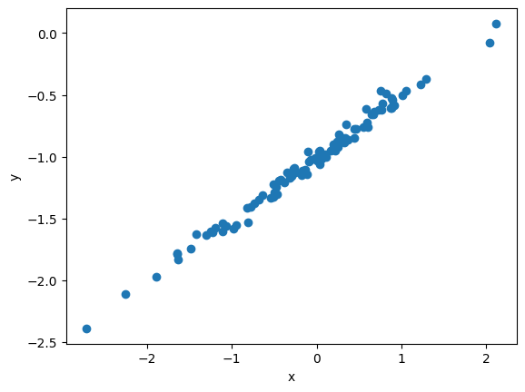
(h) Repeat (a)–(f) after modifying the data generation process in such a way that there is less noise in the data. The model (3.39) should remain the same. You can do this by decreasing the variance of the normal distribution used to generate the error term \(\epsilon\) in (b). Describe your results.

# (h) and (i_ could be done using a function to save space but I noticed 
# that pretty late  because I messed up the order and had to reorder them later

eps = rng.normal(0, 0.05, size=100)
y = -1 + 0.5 * x + eps
plt.scatter(x, y)
plt.xlabel('x')
plt.ylabel('y');

df = pd.DataFrame({'x': x, 'y':y})
X = MS('x').fit_transform(df)
less_noisy = sm.OLS(y, X).fit()
summarize(less_noisy)

	coef	std err	t	P>|t|
intercept	-1.0081	0.005	-217.791	0.0
x	0.4994	0.005	92.211	0.0

_, ax = plt.subplots(figsize=(8,6))
ax.scatter(x, y, marker='o', facecolors='none', edgecolors='black', linewidths=0.5, label='population')
ax.set_xlabel('x')
ax.set_ylabel('y')

intercept, slope = less_noisy.params
xlim = ax.get_xlim()
ylim = [intercept + xlim[0] * slope, intercept + xlim[1] * slope]
ax.plot(xlim, ylim, linewidth=2, color='orange', label='Least Squares Line')
ax.legend();

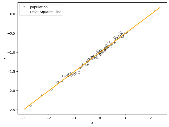
We can see that the predicted coefficients are even closer to their true values now that there’s less noise in the data and standard error is very miniscule.

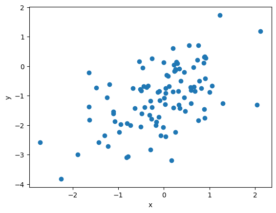
(i) Repeat (a)–(f) after modifying the data generation process in such a way that there is more noise in the data. The model (3.39) should remain the same. You can do this by increasing the variance of the normal distribution used to generate the error term \(\epsilon\) in (b). Describe your results.

eps = rng.normal(0, 1, size=100)
y = -1 + 0.5 * x + eps
plt.scatter(x, y)
plt.xlabel('x')
plt.ylabel('y');

df = pd.DataFrame({'x': x, 'y':y})
X = MS('x').fit_transform(df)
noisy = sm.OLS(y, X).fit()
summarize(noisy)

	coef	std err	t	P>|t|
intercept	-1.0092	0.087	-11.539	0.0
x	0.6470	0.102	6.323	0.0

_, ax = plt.subplots(figsize=(8,6))
ax.scatter(x, y, marker='o', facecolors='none', edgecolors='black', linewidths=0.5, label='population')
ax.set_xlabel('x')
ax.set_ylabel('y')

intercept, slope = noisy.params
xlim = ax.get_xlim()
ylim = [intercept + xlim[0] * slope, intercept + xlim[1] * slope]
ax.plot(xlim, ylim, linewidth=2, color='orange', label='Least Squares Line')
ax.legend();

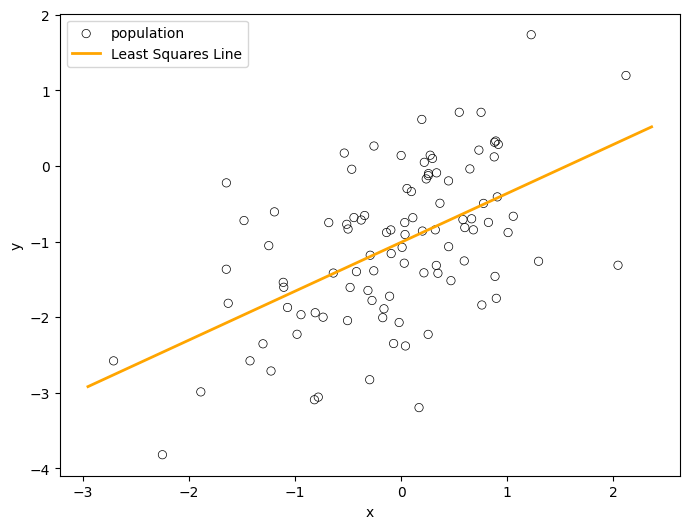
We can see that the predicted coefficients are even farther from their true values now that there’s more noise in the data and standard error is much bigger than before.

(j) What are the confidence intervals for β 0 and β 1 based on the original data set, the noisier data set, and the less noisy dataset? Comment on your results.

results.conf_int(alpha=0.05)

	0	1
intercept	-1.068891	-0.969122
x	0.433783	0.550508

less_noisy.conf_int(alpha=0.05)

	0	1
intercept	-1.017282	-0.998911
x	0.488614	0.510108

noisy.conf_int(alpha=0.05)

	0	1
intercept	-1.182711	-0.835607
x	0.443946	0.850043

We can see that the noisier the data set the wider the confidence interval it has which makes sense since standard error increases with noise and confidence intervals are calculated using the following approximation:

\[ \hat\beta \pm 2 \cdot SE(\hat\beta) \]

Q14.

This problem focuses on the collinearity problem.

(a) Perform the following commands in Python.

rng = np.random.default_rng (10)
x1 = rng.uniform(0, 1, size =100)
x2 = 0.5 * x1 + rng.normal(size =100) / 10
y = 2 + 2 * x1 + 0.3 * x2 + rng.normal(size =100)

The last line corresponds to creating a linear model in which y is a function of x1 and x2. Write out the form of the linear model. What are the regression coefficients?

The linear model takes this form:

\[ Y = 2 + 2 X_1 + 0.3 X_2 + \epsilon \]

and the coefficients are:

\[\begin{split} \begin{aligned} \beta_0 = 2 \\ \beta_1 = 2 \\ \beta_2 = 0.3 \end{aligned} \end{split}\]

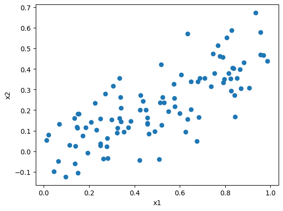
(b) What is the correlation between x1 and x2? Create a scatterplot displaying the relationship between the variables

np.corrcoef(x1, x2)

array([[1.       , 0.7723245],
       [0.7723245, 1.       ]])

plt.scatter(x1, x2)
plt.xlabel('x1')
plt.ylabel('x2');

(c) Using this data, fit a least squares regression to predict y using x1 and x2. Describe the results obtained. What are \(\hat\beta_0\), \(\hat\beta_1\), and \(\hat\beta_2\)? How do these relate to the true \(\beta_0\), \(\beta_1\), and \(\beta_2\)? Can you reject the null hypothesis \(H_0 : \beta_1 = 0\)? How about the null hypothesis \(H_0 : \beta_2 = 0\)?

df = pd.DataFrame({'x1': x1, 'x2':x2, 'y':y})
X = MS(['x1', 'x2']).fit_transform(df)
results = sm.OLS(y, X).fit()
summarize(results)

	coef	std err	t	P>|t|
intercept	1.9579	0.190	10.319	0.000
x1	1.6154	0.527	3.065	0.003
x2	0.9428	0.831	1.134	0.259

The predicted coefficient values are:

\[\begin{split} \begin{aligned} \hat\beta_0 = 1.9579 \\ \hat\beta_1 = 1.6154 \\ \hat\beta_2 = 0.9428 \end{aligned} \end{split}\]

The predicted coefficient for the intercept is pretty close to the real value however the other predicted coefficients happen to fall pretty far from their real values.

We can reject the null hypothesis \(H_0 : \beta_1 = 0\) because of its small p-value but fail to reject \(H_0 : \beta_2 = 0\) because its p-value isn’t statistically significant at 0.259.

(d) Now fit a least squares regression to predict y using only x1. Comment on your results. Can you reject the null hypothesis \(H_0 : \beta_1 = 0\)?

df = pd.DataFrame({'x1': x1, 'x2':x2, 'y':y})
X = MS(['x1']).fit_transform(df)
results = sm.OLS(y, X).fit()
summarize(results)

	coef	std err	t	P>|t|
intercept	1.9371	0.189	10.242	0.0
x1	2.0771	0.335	6.196	0.0

The predicted coefficient values are closer to their true values. Yes we can reject the null hypothesis \(H_0 : \beta_1 = 0\) due to the low associated p-value.

(e) Now fit a least squares regression to predict y using only x2. Comment on your results. Can you reject the null hypothesis \(H_0 : \beta_1 = 0\)?

df = pd.DataFrame({'x1': x1, 'x2':x2, 'y':y})
X = MS(['x2']).fit_transform(df)
results = sm.OLS(y, X).fit()
summarize(results)

	coef	std err	t	P>|t|
intercept	2.3239	0.154	15.124	0.0
x2	2.9103	0.550	5.291	0.0

There’s a considerable difference between the predicted coefficients and thier true values. Though we can reject the null hypothesis \(H_0 : \beta_1 = 0\) here because the p-value is pretty small.

(f) Do the results obtained in (c)–(e) contradict each other? Explain your answer.

They don’t because in the presence of x1 the variable x2 has less explanatory power due to it being a function of x1 which is the reason we failed to reject the null then.

However while fitting y on x2 in the absence of x1, the relationship between them is the only thing the model can rely on to fit the data and there’s clearly a strong relationship hence it’d result in us rejecting the null (low p-value).

This is also the model written in terms of either variable which shows us that the coefficients values are when fitted seperately are reasonable.

\[\begin{split} Y = 2 + 2.15 X_1 + 1.03 \epsilon \\ \end{split}\]

\[ Y = 2 + 4.3 X_2 + 0.6 \epsilon \]

(g) Suppose we obtain one additional observation, which was unfortunately mismeasured. We use the function np.concatenate to add this additional observation to each of x1, x2 and y.

x1 = np.concatenate ([x1 , [0.1]])
x2 = np.concatenate ([x2 , [0.8]])
y = np.concatenate ([y, [6]])

Re-fit the linear models from (c) to (e) using this new data. What effect does this new observation have on the each of the models? In each model, is this observation an outlier? A high-leverage point? Both? Explain your answers.

def fit_and_diagplot(predictor_list):
    with sns.axes_style("darkgrid") :
        df = pd.DataFrame({'x1': x1, 'x2':x2, 'y':y})
        X = MS(predictor_list).fit_transform(df)
        results = sm.OLS(y, X).fit()
        
        fig, axes = plt.subplots(1, 2, figsize=(13, 6))
        
        full_name = ','.join(predictor_list)
        fig.suptitle(f'y onto {full_name}')
        
        # plot the new outlier point
        outlier_index = 100
        axes[0].scatter(results.fittedvalues[outlier_index], results.resid[outlier_index], c='r', alpha=1)
        
        sns.residplot(x=results.fittedvalues, y=y,
                    lowess=True,
                    scatter_kws={'alpha': 0.5},
                    line_kws={'color': 'red', 'lw': 1, 'alpha': 0.5},
                    ax=axes[0])
        axes[0].set_xlabel('Fitted Values')
        axes[0].set_ylabel('Residuals')
        axes[0].axhline(0, ls=':', color='k');
        
        
        infl = results.get_influence()
        
        axes[1].scatter(np.arange(X.shape[0])[outlier_index], infl.hat_matrix_diag[outlier_index], c='r', alpha=1)
        
        axes[1].scatter(np.arange(X.shape[0]), infl.hat_matrix_diag, marker='o', facecolors='none', edgecolors='black', linewidths=0.5)
        
        h_avg = ((X.shape[1]+1)/X.shape[0])
        axes[1].axhline(h_avg, ls='--', c='r', alpha=0.6, label='Average Leverage')
        axes[1].set_xlabel('Index')
        axes[1].set_ylabel('Leverage')
        axes[1].legend()
        print(f'Index of highest leverage point: {np.argmax(infl.hat_matrix_diag)}')
        print(f'Value of highest leverage point: {X.iloc[np.argmax(infl.hat_matrix_diag)]}')
        
        for ax in axes: 
            for spine in ax.spines.values():
                spine.set_visible(True)
                spine.set_linewidth(1)
                spine.set_color('black');
        
        
        return summarize(results)

# Model (c)
fit_and_diagplot(['x1', 'x2'])

Index of highest leverage point: 100
Value of highest leverage point: intercept    1.0
x1           0.1
x2           0.8
Name: 100, dtype: float64

	coef	std err	t	P>|t|
intercept	2.0618	0.192	10.720	0.000
x1	0.8575	0.466	1.838	0.069
x2	2.2663	0.705	3.216	0.002

# Model (d)
fit_and_diagplot(['x1'])

Index of highest leverage point: 52
Value of highest leverage point: intercept    1.000000
x1           0.987124
Name: 52, dtype: float64

	coef	std err	t	P>|t|
intercept	2.0739	0.201	10.310	0.0
x1	1.8760	0.358	5.236	0.0

# Model (e)
fit_and_diagplot(['x2'])

Index of highest leverage point: 100
Value of highest leverage point: intercept    1.0
x2           0.8
Name: 100, dtype: float64

	coef	std err	t	P>|t|
intercept	2.2840	0.151	15.088	0.0
x2	3.1458	0.524	6.008	0.0

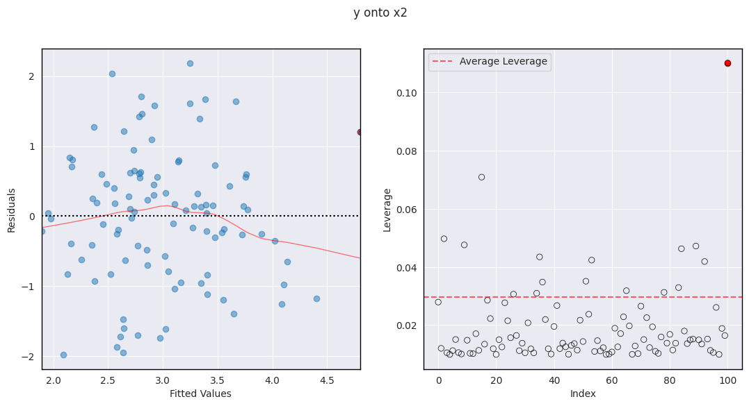
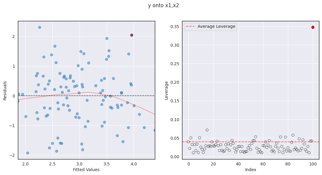
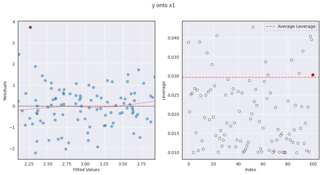
I plotted the new added point in red to highlight it.

Model (c) y onto x1 and x2:

We can see that the hypothesis \(H_0: \beta_1 = 0\) is no longer statistically significant at any conventional confidence level and \(H_0: \beta_2 = 0\) became statistically significant after adding that point. And comparing the new and old coefficients we can tell that the new \(\beta_1\) is much less than the old one but the opposite is true for \(\beta_2\).

We can also see from the residuals and leverage plots that this point isn’t necessarily an outlier however it has extremely high leverage which is why it heavily affected our model.

Model (d) y onto x1:

Not much changed with this model. Looking at the residuals and leverage plots we can see that the point is a potential outlier since it has the highest residual but it also has very average leverage here.

Model (e) y onto x2:

We can see a slight increase in the coefficients but no notable changes there. Looking at the residuals and leverage plots we can see that the point isn’t an outlier but has a very high leverage.

Q15.

This problem involves the Boston data set, which we saw in the lab for this chapter. We will now try to predict per capita crime rate using the other variables in this data set. In other words, per capita crime rate is the response, and the other variables are the predictors.

Note: I kinda gave up here just tried to get this question over with

(a) For each predictor, fit a simple linear regression model to predict the response. Describe your results. In which of the models is there a statistically significant association between the predictor and the response? Create some plots to back up your assertions.

boston = load_data('Boston')
boston.head()

	crim	zn	indus	chas	nox	rm	age	dis	rad	tax	ptratio	lstat	medv
0	0.00632	18.0	2.31	0	0.538	6.575	65.2	4.0900	1	296	15.3	4.98	24.0
1	0.02731	0.0	7.07	0	0.469	6.421	78.9	4.9671	2	242	17.8	9.14	21.6
2	0.02729	0.0	7.07	0	0.469	7.185	61.1	4.9671	2	242	17.8	4.03	34.7
3	0.03237	0.0	2.18	0	0.458	6.998	45.8	6.0622	3	222	18.7	2.94	33.4
4	0.06905	0.0	2.18	0	0.458	7.147	54.2	6.0622	3	222	18.7	5.33	36.2

boston.info()

<class 'pandas.core.frame.DataFrame'>
RangeIndex: 506 entries, 0 to 505
Data columns (total 13 columns):
 #   Column   Non-Null Count  Dtype  
---  ------   --------------  -----  
 0   crim     506 non-null    float64
 1   zn       506 non-null    float64
 2   indus    506 non-null    float64
 3   chas     506 non-null    int64  
 4   nox      506 non-null    float64
 5   rm       506 non-null    float64
 6   age      506 non-null    float64
 7   dis      506 non-null    float64
 8   rad      506 non-null    int64  
 9   tax      506 non-null    int64  
 10  ptratio  506 non-null    float64
 11  lstat    506 non-null    float64
 12  medv     506 non-null    float64
dtypes: float64(10), int64(3)
memory usage: 51.5 KB

y = boston['crim']
predictors = boston.columns.drop('crim')

# Create subplots
fig, axes = plt.subplots(nrows=3, ncols=4, figsize=(20, 12))
axes = axes.flatten()

coefficients_univariate = []
for i, predictor in enumerate(predictors):
    X = MS([predictor]).fit_transform(boston)
    results = sm.OLS(y, X).fit()
    coefficients_univariate.append(results.params.iloc[1])
    print(summarize(results))
    
    # Plot on the corresponding subplot
    axes[i].scatter(boston[predictor], y)
    axes[i].set_xlabel(predictor)
    axes[i].set_ylabel('crim')
    print()

plt.tight_layout()
plt.show()

             coef  std err       t  P>|t|
intercept  4.4537    0.417  10.675    0.0
zn        -0.0739    0.016  -4.594    0.0

             coef  std err      t  P>|t|
intercept -2.0637    0.667 -3.093  0.002
indus      0.5098    0.051  9.991  0.000

             coef  std err      t  P>|t|
intercept  3.7444    0.396  9.453  0.000
chas      -1.8928    1.506 -1.257  0.209

              coef  std err       t  P>|t|
intercept -13.7199    1.699  -8.073    0.0
nox        31.2485    2.999  10.419    0.0

              coef  std err      t  P>|t|
intercept  20.4818    3.364  6.088    0.0
rm         -2.6841    0.532 -5.045    0.0

             coef  std err      t  P>|t|
intercept -3.7779    0.944 -4.002    0.0
age        0.1078    0.013  8.463    0.0

             coef  std err       t  P>|t|
intercept  9.4993    0.730  13.006    0.0
dis       -1.5509    0.168  -9.213    0.0

             coef  std err       t  P>|t|
intercept -2.2872    0.443  -5.157    0.0
rad        0.6179    0.034  17.998    0.0

             coef  std err       t  P>|t|
intercept -8.5284    0.816 -10.454    0.0
tax        0.0297    0.002  16.099    0.0

              coef  std err      t  P>|t|
intercept -17.6469    3.147 -5.607    0.0
ptratio     1.1520    0.169  6.801    0.0

             coef  std err       t  P>|t|
intercept -3.3305    0.694  -4.801    0.0
lstat      0.5488    0.048  11.491    0.0

              coef  std err       t  P>|t|
intercept  11.7965    0.934  12.628    0.0
medv       -0.3632    0.038  -9.460    0.0

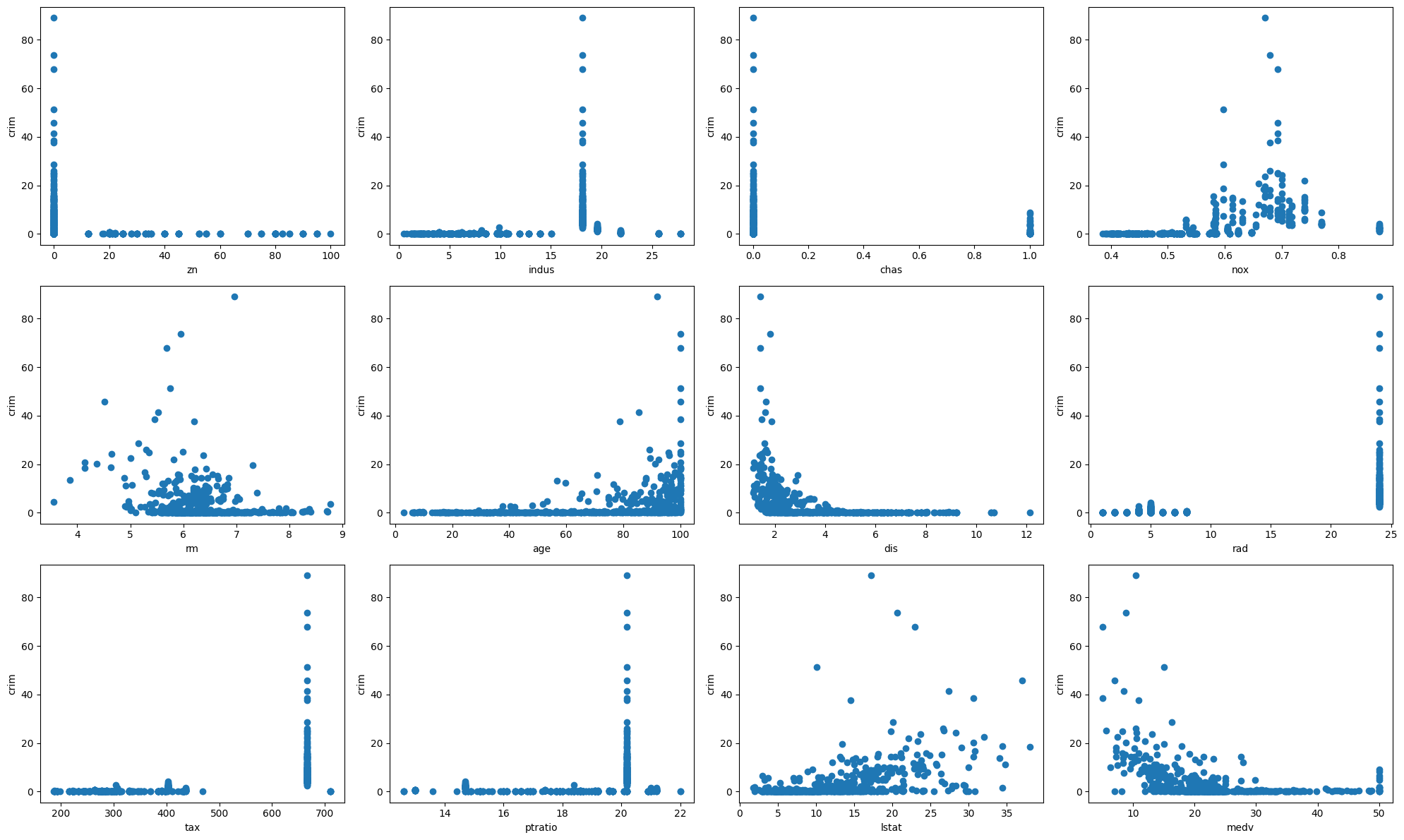
Looking at the p-values the relationships between each of the predictors and the response crim, in the absence of others is statistically significant apart from chas which has a p-value of 0.209

coefficients_univariate

[-0.07393497740412348,
 0.5097763311042313,
 -1.8927765508037608,
 31.248531201122923,
 -2.684051224113948,
 0.10778622713953308,
 -1.5509016824100994,
 0.6179109273272014,
 0.029742252822765353,
 1.1519827870705868,
 0.5488047820623981,
 -0.363159922257603]

(b) Fit a multiple regression model to predict the response using all of the predictors. Describe your results. For which predictors can we reject the null hypothesis \(H_0 : \beta_j = 0\)?

y = boston['crim']
X = MS(predictors).fit_transform(boston)
results = sm.OLS(y, X).fit()
summarize(results)

	coef	std err	t	P>|t|
intercept	13.7784	7.082	1.946	0.052
zn	0.0457	0.019	2.433	0.015
indus	-0.0584	0.084	-0.698	0.486
chas	-0.8254	1.183	-0.697	0.486
nox	-9.9576	5.290	-1.882	0.060
rm	0.6289	0.607	1.036	0.301
age	-0.0008	0.018	-0.047	0.962
dis	-1.0122	0.282	-3.584	0.000
rad	0.6125	0.088	6.997	0.000
tax	-0.0038	0.005	-0.730	0.466
ptratio	-0.3041	0.186	-1.632	0.103
lstat	0.1388	0.076	1.833	0.067
medv	-0.2201	0.060	-3.678	0.000

We can reject the null hypothesis for rad, medv, dis at a 0.1% confidence level, and zn at a 5% confidence level. We fail to reject it for the rest of the predictors though.

(c) How do your results from (a) compare to your results from (b)? Create a plot displaying the univariate regression coefficients from (a) on the \(x\)-axis, and the multiple regression coefficients from (b) on the \(y\)-axis. That is, each predictor is displayed as asingle point in the plot. Its coefficient in a simple linear regression model is shown on the \(x\)-axis, and its coefficient estimate in the multiple linear regression model is shown on the \(y\)-axis.

The results varied greatly, for the univariate regressions we rejected all the null hypotheses apart from one, however for the multiple regression we rejected only 4 and failed to reject the rest.

plt.scatter(coefficients_univariate, results.params.iloc[1:], marker='o', facecolors='orange', edgecolors='black', linewidths=0.5);
plt.xlabel('Univariate Regression Coefficients')
plt.ylabel('Multiple Regression Coefficients');

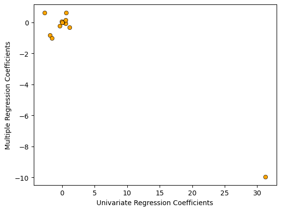
It’s also interesting to note that the coefficients for nox were extremely high in both cases but of opposite signs. Highly positive in the univariate case (+31.2485) in the absence of other predictors, and highly negative in the multiple regression case (-9.9576) in the presence of the other predictors.

(d) Is there evidence of non-linear association between any of the predictors and the response? To answer this question, for each predictor \(X\), fit a model of the form:

\[ Y = \beta_0 + \beta_1 X + \beta_2 X^2 + \beta_3 X^3 + \epsilon \]

y = boston['crim']
for predictor in predictors:
    X = MS([poly(predictor, degree=3)]).fit_transform(boston)
    results = sm.OLS(y, X).fit()
    coefficients_univariate.append(results.params.iloc[1])
    print(summarize(results))
    print()

                          coef  std err      t  P>|t|
intercept               3.6135    0.372  9.709  0.000
poly(zn, degree=3)[0] -38.7498    8.372 -4.628  0.000
poly(zn, degree=3)[1]  23.9398    8.372  2.859  0.004
poly(zn, degree=3)[2] -10.0719    8.372 -1.203  0.230

                             coef  std err       t  P>|t|
intercept                  3.6135    0.330  10.950  0.000
poly(indus, degree=3)[0]  78.5908    7.423  10.587  0.000
poly(indus, degree=3)[1] -24.3948    7.423  -3.286  0.001
poly(indus, degree=3)[2] -54.1298    7.423  -7.292  0.000

                           coef  std err      t  P>|t|
intercept                3.6927    0.388  9.505  0.000
poly(chas, degree=3)[0] -0.1178    0.066 -1.784  0.075
poly(chas, degree=3)[1] -0.5757    0.234 -2.460  0.014
poly(chas, degree=3)[2] -0.7966    0.708 -1.125  0.261

                           coef  std err       t  P>|t|
intercept                3.6135    0.322  11.237    0.0
poly(nox, degree=3)[0]  81.3720    7.234  11.249    0.0
poly(nox, degree=3)[1] -28.8286    7.234  -3.985    0.0
poly(nox, degree=3)[2] -60.3619    7.234  -8.345    0.0

                          coef  std err      t  P>|t|
intercept               3.6135     0.37  9.758  0.000
poly(rm, degree=3)[0] -42.3794     8.33 -5.088  0.000
poly(rm, degree=3)[1]  26.5768     8.33  3.191  0.002
poly(rm, degree=3)[2]  -5.5103     8.33 -0.662  0.509

                           coef  std err       t  P>|t|
intercept                3.6135    0.349  10.368  0.000
poly(age, degree=3)[0]  68.1820    7.840   8.697  0.000
poly(age, degree=3)[1]  37.4845    7.840   4.781  0.000
poly(age, degree=3)[2]  21.3532    7.840   2.724  0.007

                           coef  std err       t  P>|t|
intercept                3.6135    0.326  11.087    0.0
poly(dis, degree=3)[0] -73.3886    7.331 -10.010    0.0
poly(dis, degree=3)[1]  56.3730    7.331   7.689    0.0
poly(dis, degree=3)[2] -42.6219    7.331  -5.814    0.0

                            coef  std err       t  P>|t|
intercept                 3.6135    0.297  12.164  0.000
poly(rad, degree=3)[0]  120.9074    6.682  18.093  0.000
poly(rad, degree=3)[1]   17.4923    6.682   2.618  0.009
poly(rad, degree=3)[2]    4.6985    6.682   0.703  0.482

                            coef  std err       t  P>|t|
intercept                 3.6135    0.305  11.860  0.000
poly(tax, degree=3)[0]  112.6458    6.854  16.436  0.000
poly(tax, degree=3)[1]   32.0873    6.854   4.682  0.000
poly(tax, degree=3)[2]   -7.9968    6.854  -1.167  0.244

                               coef  std err       t  P>|t|
intercept                    3.6135    0.361  10.008  0.000
poly(ptratio, degree=3)[0]  56.0452    8.122   6.901  0.000
poly(ptratio, degree=3)[1]  24.7748    8.122   3.050  0.002
poly(ptratio, degree=3)[2] -22.2797    8.122  -2.743  0.006

                             coef  std err       t  P>|t|
intercept                  3.6135    0.339  10.654  0.000
poly(lstat, degree=3)[0]  88.0697    7.629  11.543  0.000
poly(lstat, degree=3)[1]  15.8882    7.629   2.082  0.038
poly(lstat, degree=3)[2] -11.5740    7.629  -1.517  0.130

                            coef  std err       t  P>|t|
intercept                 3.6135    0.292  12.374    0.0
poly(medv, degree=3)[0] -75.0576    6.569 -11.426    0.0
poly(medv, degree=3)[1]  88.0862    6.569  13.409    0.0
poly(medv, degree=3)[2] -48.0334    6.569  -7.312    0.0

There seems to be strong evidence of non-linearity considering the quadratic term is significant in a lot of the models, and even the cubic term seems to be statstically significant in a few others.