Ch8: Tree-Based Methods

import numpy as np
import pandas as pd
import matplotlib.pyplot as plt
import seaborn as sns

sns.set_theme()

%matplotlib inline

import sklearn.model_selection as skm
import sklearn.linear_model as skl

from sklearn.pipeline import Pipeline
from sklearn.preprocessing import StandardScaler

from sklearn.neighbors import KNeighborsClassifier as KNN
from sklearn.tree import (DecisionTreeClassifier as DTC,
                          DecisionTreeRegressor as DTR,
                          plot_tree,
                          export_text)

from sklearn.metrics import (accuracy_score,
                             precision_score,
                             recall_score,
                             make_scorer)

from sklearn.ensemble import \
     (RandomForestRegressor as RF,
      GradientBoostingRegressor as GBR,
      GradientBoostingClassifier as GBC)
     
from ISLP.bart import BART

from ISLP import load_data, confusion_table
from ISLP.models import ModelSpec as MS

Conceptual

Q1.

We’ll create a sketch with arbitrarily chosen cut points,

\[ t_1 = 3,\quad t_2 = 40,\quad t_3 = 80 \]

\[ t_4 = -9,\quad t_5 =12 \]

with plt.xkcd():
    plt.rcParams['font.family'] = 'DejaVu Sans' # to get rid of xkcd font warnings
    _, ax = plt.subplots(figsize=(8, 6))
    rng = np.random.default_rng(12)
    x = rng.uniform(-20, 20, 200)
    y = rng.uniform(0, 100, 200)
    
    sns.scatterplot(x=x, y=y, ax=ax, c='black', alpha=0.7)
    ax.set_xlabel('x')
    ax.set_ylabel('y')
    
    # 5 cuts
    t1 = 3 
    t2 = 40
    t3 = 80
    t4 = -9
    t5 = 12
    
    xlim = ax.get_xlim()
    ylim = ax.get_ylim()
    xrange = xlim[1] - xlim[0]
    yrange = ylim[1] - ylim[0]
     
    ax.axvline(t1, label='t1', c='r')
    ax.axhline(t2, xmax=(t1+xlim[1])/xrange, label='t2', c='b')
    ax.axhline(t3, xmin=(t1+xlim[1])/xrange, label='t3', c='b')
    ax.axvline(t4, ymin=(t2-ylim[0])/yrange, label='t4', c='r')
    ax.axvline(t5, ymax=(t3-ylim[0])/yrange, label='t5', c='r')
    
    # Annotate where the lines cut the axes:
    # For vertical lines
    ax.text(t1, ylim[0], f'$t_1={t1}$', ha='center', va='top', color='k')
    ax.text(t4, ylim[1], f'$t_4={t4}$', ha='center', va='top', color='k')
    ax.text(t5, ylim[0], f'$t_5={t5}$', ha='center', va='top', color='k')
    
    # For horizontal lines
    ax.text(xlim[0], t2, f'$t_2={t2}$', rotation=90, ha='left', va='center', color='k')
    ax.text(xlim[1], t3, f'$t_3={t3}$', rotation=90, ha='left', va='center', color='k')
    
    
    # Annotate regions
    ax.text(0.25, 0.2, 'R1', c='purple', transform=ax.transAxes)
    ax.text(0.1, 0.7, 'R2', c='purple', transform=ax.transAxes)
    ax.text(0.4, 0.7, 'R3', c='purple', transform=ax.transAxes)
    
    ax.text(0.65, 0.3, 'R4', c='purple', transform=ax.transAxes)
    ax.text(0.85, 0.3, 'R5', c='purple', transform=ax.transAxes)
    ax.text(0.75, 0.8, 'R6', c='purple', transform=ax.transAxes)

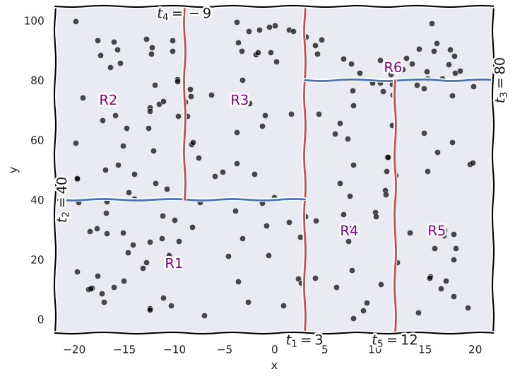
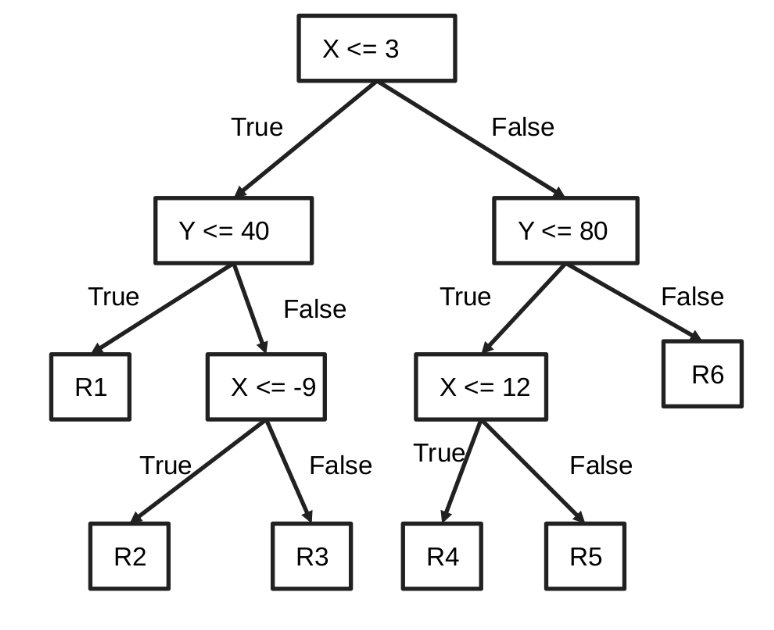
And the corresponding decision tree.

Q2.

Starting with equation (8.12):

\[ \hat f(x) = \sum_{b = 1}^{B} \lambda \hat f^b(x) \]

Since the number of splits is \(1\), every tree (or stump in this case) makes a binary decision on one variable \(X_j\), hence every model \(\hat f^b(x)\) above can be written as the sum of binary models that take the form:

\[\begin{split} f_j(X_j) = \begin{cases} A_j, & \text{if } X_j \le t_j\\ B_j, & \text{if } X_j \gt t_j \end{cases} \end{split}\]

Where \(A_j\) and \(B_j\) are arbitrary decisions for the \(j\text{th}\) predictor, and \(t_j\) is an arbitrary cut point.

And since the number of splits \(d = 1\), for every iteration \(b\) while fitting the boosting model, the \(p\) functions above would all be \(0\) except for the one chosen by the model.

\[ \hat f^b(X) = \sum_{j = 1}^{p} \hat f^b_j(X_j) \]

Where \(\hat f^b_j(X_j) \) is the model in the \(b\text{th}\) iteration that picked the \(j\text{th}\) predictor. This would of course just be \(\hat f_j(X_j)\) for some choice of \(j\) in \([1, p]\).

Then substituing in (8.12)

\[ \hat f(X) = \sum_{b = 1}^{B} \lambda \sum_{j = 1}^{p} \hat f^b_j(X_j) \]

And summing up over all iterations while keeping the models for each predictor seperate we get:

\[ \hat f(X) = \sum_{j = 1}^{p} \hat f_j(X_j) \]

Q3.

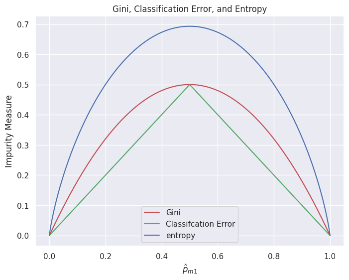
We can solve this by doing a math derivation and substituing for \(\hat p_{m1} = 1 - \hat p_{m2}\), which makes the equations we have to plot simpler but it ultimately leads to the same result, so we’ll just use the original equations with some numpy magic.

p1 = np.linspace(0.00000001, 0.99999999, 1000) # Not using 0 and 1 to avoid problems with np.log 
p = np.column_stack((p1, 1 - p1))

G = np.sum(p * (1-p), axis=1)
E = 1 - np.maximum(p1, 1 - p1)
D = -np.sum(p*np.log(p), axis=1)

fig, ax = plt.subplots(figsize=(8,6))
ax.plot(p1, G, c='r', label='Gini')
ax.plot(p1, E, c='g', label='Classifcation Error')
ax.plot(p1, D, c='b', label='entropy')

ax.set_xlabel('$\hat p_{m1}$')
ax.set_ylabel('Impurity Measure') 
ax.set_title('Gini, Classification Error, and Entropy')
ax.legend();

Q4.

(a)

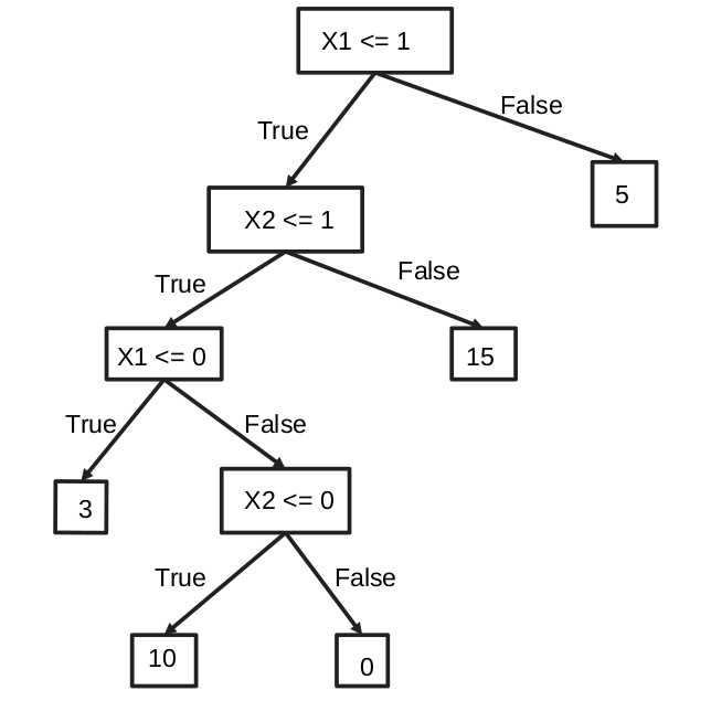
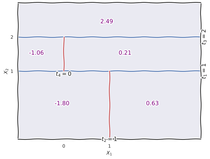
(b) We’ll reuse the code from Q1 with slight modifications to plot the regions.

with plt.xkcd():
    plt.rcParams['font.family'] = 'DejaVu Sans' # to get rid of xkcd font warnings
    _, ax = plt.subplots(figsize=(8,6))
    rng = np.random.default_rng(12)
    x1 = rng.uniform(0, 2, 200)
    x2 = rng.uniform(0, 2, 200)
    
    ax.set_xlabel('$X_1$')
    ax.set_ylabel('$X_2$')
    
    # 5 cuts
    t1 = 1
    t2 = 1
    t3 = 2
    t4 = 0
    
    ax.set_xticks([0, 1])
    ax.set_yticks([1, 2])
    xlim = [-1, 3]
    ylim = [-1, 3]
    ax.set_xlim(xlim)
    ax.set_ylim(ylim)
    xrange = xlim[1] - xlim[0]
    yrange = ylim[1] - ylim[0]
     
    ax.axhline(t1, label='t1', c='b')
    ax.axvline(t2, ymax=(t1-ylim[0])/yrange, label='t2', c='r')
    ax.axhline(t3, label='t3', c='b')
    ax.axvline(t4, ymin=(t1-ylim[0])/yrange,ymax=(t3-ylim[0])/yrange, label='t4', c='r')
    
    # Annotate where the lines cut the axes:
    # For vertical lines
    ax.text(t2, ylim[0], f'$t_2={t2}$', ha='center', va='center', color='k')
    ax.text(t4, t2, f'$t_4={t4}$', ha='center', va='top', color='k')    
    
    # For horizontal lines
    ax.text(xlim[1], t2, f'$t_1={t1}$', rotation=90, ha='left', va='center', color='k')
    ax.text(xlim[1], t3, f'$t_3={t3}$', rotation=90, ha='left', va='center', color='k')
    

    # Annotate regions
    ax.text(0.2, 0.25, '-1.80', c='purple', transform=ax.transAxes)
    ax.text(0.7, 0.25, '0.63', c='purple', transform=ax.transAxes)
    ax.text(0.45, 0.85, '2.49', c='purple', transform=ax.transAxes)
    ax.text(0.06, 0.62, '-1.06', c='purple', transform=ax.transAxes)
    ax.text(0.55, 0.62, '0.21', c='purple', transform=ax.transAxes)
    

Q5.

p =  np.array([0.1, 0.15, 0.2, 0.2, 0.55, 0.6, 0.6, 0.65, 0.7, 0.75])
p

array([0.1 , 0.15, 0.2 , 0.2 , 0.55, 0.6 , 0.6 , 0.65, 0.7 , 0.75])

We’ll classify according to majority vote first, any probability greater than \(0.5\) classifies as Red (\(1\)).

vote = np.where(p > 0.5, 1, 0)
np.unique(vote, return_counts=True)

(array([0, 1]), array([4, 6]))

\(6\) votes for Red and \(4\) votes for Green. Hence the classifer based on majority vote would pick Red for this value of \(X\).

Now we’ll classify according to the average probability.

p.mean()

0.45

The average probability is \(0.45\) which means the classifier would pick Green given this value of \(X\).

Q6.

We’ll start with Algorithm 8.1 from the book for building a regression tree and expand on the details in each step:

1. Use recursive binary splitting to grow a large tree on the training data, stopping only when each terminal node has fewer than some minimum number of observations.

   1. Start at the root node (the entire dataset).

   2. Chose a splitting point as follows:

      1. For each predictor and for every possible split point along that predictor, split the data into two regions:

         • Left, where it contains predictor values less than the splitting point.

         • Right, where it contains predictor values greater than the splitting point.

      2. Calculate the sum of squared errors (SSEs) for both regions for every splitting point and predictor used:

      \[ SSE_{split} = \sum_{i \in L} (y_i - \bar y_{L})^2 + \sum_{i \in R} (y_i - \bar y_{R})^2 \]

      • \(R\): region on the right.

      • \(L\): region on the left.

      • \(y_i\): observed response.

      • \(\bar y_{L}\) and \(\bar y_{R}\): the average of the response values in the left and right regions respectively.

      3. Chose the split (predictor and point) that minimizes the SSE.

   3. Perform the chosen split on the data and append the two regions as left and right nodes to the root node.

   4. Recursion:

      1. Perform the same process (splitting and choosing a split) on every child node.

      2. Stop when each terminal node has fewer than some minimum number of observations.

2. Apply cost complexity pruning to the large tree in order to obtain a sequence of best subtrees, as a function of \(\alpha\).

   1. Start with the inital large tree \(T_0\).

   2. Repeatedly find the internal node where pruning its corresponding branch results in the smallest increase in RSS relative to number of leaves removed (n).

   \[ \alpha = \frac{\Delta Error}{n - 1} \]

   3. Prune the weakest link turning the entire branch into a terminal leaf.

   4. Store the newly pruned tree and its corresponding \(\alpha\) value and repeat the pruning process above on this smaller tree.

   5. Continue until only the root node is left. This generates a sequence of trees \((T_0, T_1, ..., T_k)\) each \(T_i\) being optimally pruned for a specific range \(\left[\alpha_i, \alpha_{i+1} \right]\).

3. Use K-fold cross-validation to choose \(\alpha\). That is, divide the training observations into \(K\) folds. For each \(k = 1, . . . , K\):

   1. Repeat Steps \(1\) and \(2\) on all but the \(k\text{th}\) fold of the training data.

   2. Evaluate the mean squared prediction error on the data in the left-out \(k\text{th}\) fold, as a function of \(\alpha\).

   3. Average the results for each value of \(\alpha\), and pick \(\alpha\) to minimize the average error.

4. Return the subtree from Step \(2\) that corresponds to the chosen value of \(\alpha\)

Applied

Q7.

boston = load_data("Boston")
boston.head()

	crim	zn	indus	chas	nox	rm	age	dis	rad	tax	ptratio	lstat	medv
0	0.00632	18.0	2.31	0	0.538	6.575	65.2	4.0900	1	296	15.3	4.98	24.0
1	0.02731	0.0	7.07	0	0.469	6.421	78.9	4.9671	2	242	17.8	9.14	21.6
2	0.02729	0.0	7.07	0	0.469	7.185	61.1	4.9671	2	242	17.8	4.03	34.7
3	0.03237	0.0	2.18	0	0.458	6.998	45.8	6.0622	3	222	18.7	2.94	33.4
4	0.06905	0.0	2.18	0	0.458	7.147	54.2	6.0622	3	222	18.7	5.33	36.2

model = MS(boston.columns.drop('medv'), intercept=False)
D = model.fit_transform(boston)
feature_names = list(D.columns)
X = np.asarray(D)
y = boston['medv']

X_train, X_test, y_train, y_test = skm.train_test_split(X, y, test_size=0.3, random_state=1)

len(feature_names)

12

We’ll fit random forest models and vary max_features from \(1\) to \(12\), and vary n_estimators from \(1\) to \(250\).

Note: this could take a few minutes to run.

test_per_m = {}
max_estimators = 250

for m in range(1, len(feature_names)+1): 
    test_per_m[m] = []
    for n in np.arange(1, max_estimators+1):
        rf_boston = RF(n_estimators=n, max_features=m, random_state=1)
        results = rf_boston.fit(X_train, y_train)
        error = np.mean((results.predict(X_test) - y_test)**2)
        test_per_m[m].append(error)

fig, ax = plt.subplots(figsize=(10, 8))
palette = sns.color_palette("viridis", len(test_per_m))

for m, test in test_per_m.items():
    
    sns.lineplot(x=np.arange(1, max_estimators),
                 y=test[1:],
                 label=f'm={m}',
                 ax=ax,
                 color=palette[m-1],
                 linewidth=1.5,
                 alpha=0.8)

# Add horizontal line at minimum error for reference
min_error = min([min(test[1:]) for test in test_per_m.values()])
ax.axhline(min_error, color='red', linestyle='--', alpha=0.5, 
           label=f'Min Error: {min_error:.4f}')

ax.set_title('Test Error by Number of Estimators', fontsize=16)
ax.set_xlabel('n_estimators')
ax.set_ylabel('MSE ')
ax.legend();

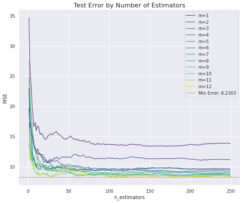
We notices that the test error doesn’t take long to stabilize, and that for low values (\(\lt 4)\) of max_features the model has significantly higher test error rates.

Q8.

carseats = load_data('Carseats')
carseats.head()

	Sales	CompPrice	Income	Advertising	Population	Price	ShelveLoc	Age	Education	Urban	US
0	9.50	138	73	11	276	120	Bad	42	17	Yes	Yes
1	11.22	111	48	16	260	83	Good	65	10	Yes	Yes
2	10.06	113	35	10	269	80	Medium	59	12	Yes	Yes
3	7.40	117	100	4	466	97	Medium	55	14	Yes	Yes
4	4.15	141	64	3	340	128	Bad	38	13	Yes	No

(a)

model = MS(carseats.columns.drop('Sales'), intercept=False)
D = model.fit_transform(carseats)
feature_names = list(D.columns)
X = np.asarray(D)
y = carseats['Sales']

X_train, X_test, y_train, y_test = skm.train_test_split(X, y, test_size=0.3, random_state=1)

(b)

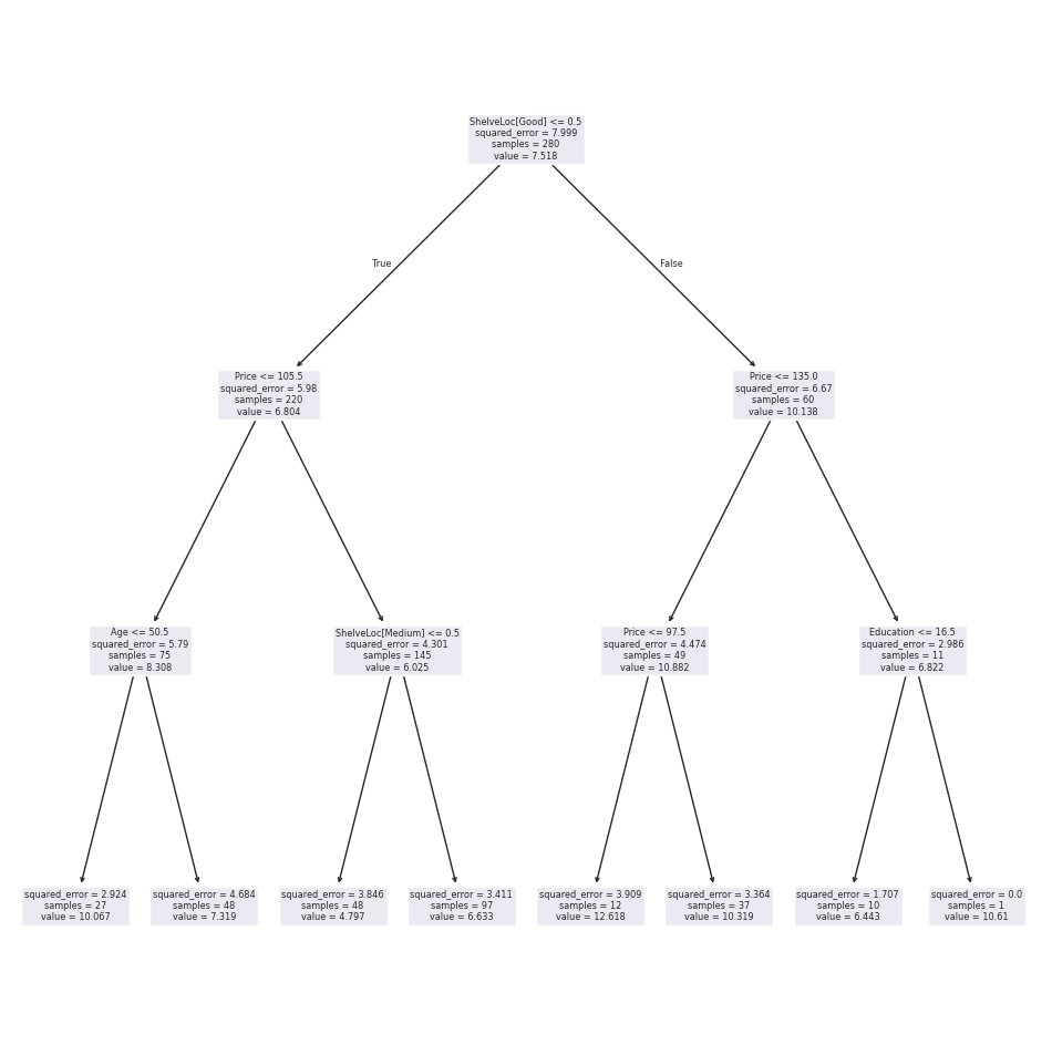
tree = DTR(max_depth=3, random_state=1)
results = tree.fit(X_train,  y_train)
plt.figure().set_size_inches(12, 12)
plot_tree(results, 
          feature_names=feature_names);

Test MSE:

np.mean((tree.predict(X_test) - y_test)**2)

4.725166009939633

(c)

kfold = skm.KFold(5,
                  shuffle=True,
                  random_state=2)

grid = skm.GridSearchCV(tree,
                        {'max_depth': np.arange(1, 20)},
                        refit=True,
                        cv=kfold,
                        scoring='neg_mean_squared_error')

G = grid.fit(X_train, y_train)
G.best_params_

{'max_depth': 3}

ccp_path = G.best_estimator_.cost_complexity_pruning_path(X_train, y_train)

grid = skm.GridSearchCV(G.best_estimator_,
                        {'ccp_alpha': ccp_path.ccp_alphas},
                        refit=True,
                        cv=kfold,
                        scoring='neg_mean_squared_error')

G = grid.fit(X_train, y_train)
G.best_params_

{'ccp_alpha': 0.0}

best_ = grid.best_estimator_
np.mean((y_test - best_.predict(X_test))**2)

4.725166009939633

No improvement from pruning the tree.

(d) Bagging:

bagging_carseats = RF(n_estimators=500,
                      max_features=X_train.shape[1],
                      random_state=1).fit(X_train, y_train)
np.mean((bagging_carseats.predict(X_test) - y_test)**2)

2.843689088653341

We got a test MSE of \(2.8437\) which is an improvement from the single regression tree.

feature_imp = pd.DataFrame(
    {'importance':bagging_carseats.feature_importances_},
    index=feature_names)
sns.barplot(feature_imp.sort_values(by='importance').T * 100/feature_imp['importance'].max(), orient='h');

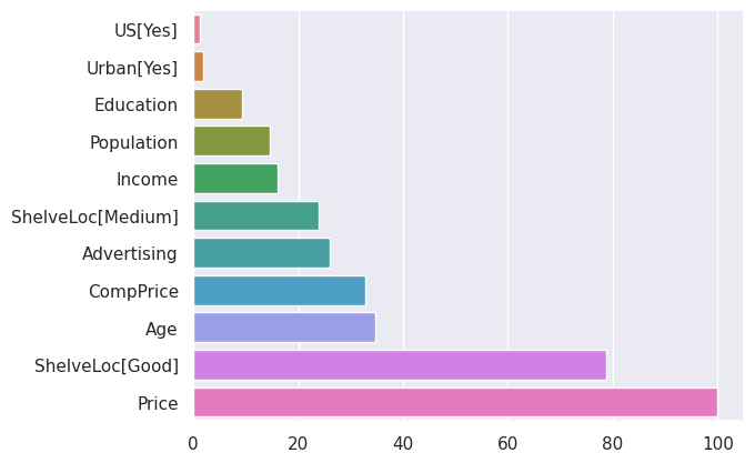
The two most important features to determine Sales are Price and ShelveLoc[Good] (indicates good quality of the shelving location for the car seats).

You can also read more about the data here.

(e) Random forests:

test_errors = []
best_rf = None
for m in np.arange(1, X_train.shape[1]+1):
    rf_carseats = RF(n_estimators=500,
                        max_features=m,
                        random_state=1).fit(X_train, y_train)
    
    error = np.mean((rf_carseats.predict(X_test) - y_test)**2)
    test_errors.append(error)
    
    if error == min(test_errors):
        best_rf = rf_carseats

fig, ax = plt.subplots(figsize=(8, 6))
sns.scatterplot(x=np.arange(1, X_train.shape[1]+1), y=test_errors, ax=ax, c='orange', marker='D')
ax.plot(np.argmin(test_errors)+1, min(test_errors), c='red', marker='D', label=f'minimum test error={min(test_errors):.4f}')
ax.set_title('RF Test Error as max_features increases for the Carseats Data', ha='center')
ax.set_xlabel('max_features')
ax.set_ylabel('Test MSE')
ax.legend();

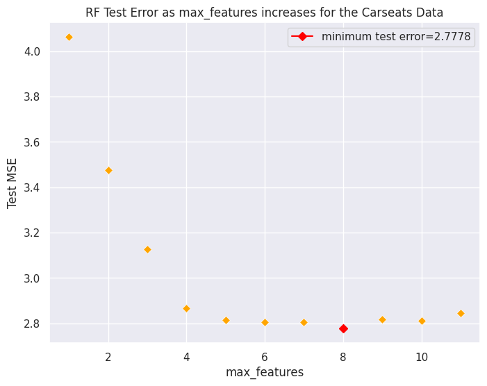
We can see that the test error rapidly decreases as max_features goes down, stabilising at around \(m = 5\) but minimized at \(8\), we also notice that it rises up a bit after \(8\) too.

feature_imp = pd.DataFrame(
    {'importance':best_rf.feature_importances_},
    index=feature_names)
sns.barplot(feature_imp.sort_values(by='importance').T * 100/feature_imp['importance'].max(), orient='h');

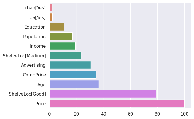
Again we see the same variables emphasized by the model.

(f) BART:

bart_carseats = BART(random_state=0, burnin=100, ndraw=1000)
bart_carseats.fit(X_train, y_train)

BART(ndraw=1000, random_state=0)

In a Jupyter environment, please rerun this cell to show the HTML representation or trust the notebook.
On GitHub, the HTML representation is unable to render, please try loading this page with nbviewer.org.

np.mean((bart_carseats.predict(X_test) - y_test)**2)

1.4032862543324767

The BART method performed even better on this data than all the previous methods.

We’ll plot the variable_inclusion means and scale them by \(100\) which can serve as measures of importance here.

var_inclusion = pd.DataFrame(
    {'inclusion':bart_carseats.variable_inclusion_.mean(0)},
    index=D.columns)
sns.barplot(var_inclusion.sort_values(by='inclusion').T * (100 / var_inclusion['inclusion'].max()), orient='h');

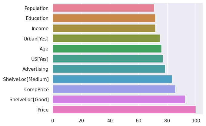
Again the model emphasized the Price and ShelveLoc[Good] variables.

Q9.

Note: decision tree algorithms are pretty sensitive to changes in random_state make sure to always have it set whether in the cross-validation folds or the tree itself.

oj = load_data('OJ')
oj.head()

	Purchase	WeekofPurchase	StoreID	PriceCH	PriceMM	DiscCH	DiscMM	SpecialCH	SpecialMM	LoyalCH	SalePriceMM	SalePriceCH	PriceDiff	Store7	PctDiscMM	PctDiscCH	ListPriceDiff	STORE
0	CH	237	1	1.75	1.99	0.00	0.0	0	0	0.500000	1.99	1.75	0.24	No	0.000000	0.000000	0.24	1
1	CH	239	1	1.75	1.99	0.00	0.3	0	1	0.600000	1.69	1.75	-0.06	No	0.150754	0.000000	0.24	1
2	CH	245	1	1.86	2.09	0.17	0.0	0	0	0.680000	2.09	1.69	0.40	No	0.000000	0.091398	0.23	1
3	MM	227	1	1.69	1.69	0.00	0.0	0	0	0.400000	1.69	1.69	0.00	No	0.000000	0.000000	0.00	1
4	CH	228	7	1.69	1.69	0.00	0.0	0	0	0.956535	1.69	1.69	0.00	Yes	0.000000	0.000000	0.00	0

oj.info()

<class 'pandas.core.frame.DataFrame'>
RangeIndex: 1070 entries, 0 to 1069
Data columns (total 18 columns):
 #   Column          Non-Null Count  Dtype   
---  ------          --------------  -----   
 0   Purchase        1070 non-null   category
 1   WeekofPurchase  1070 non-null   int64   
 2   StoreID         1070 non-null   int64   
 3   PriceCH         1070 non-null   float64 
 4   PriceMM         1070 non-null   float64 
 5   DiscCH          1070 non-null   float64 
 6   DiscMM          1070 non-null   float64 
 7   SpecialCH       1070 non-null   int64   
 8   SpecialMM       1070 non-null   int64   
 9   LoyalCH         1070 non-null   float64 
 10  SalePriceMM     1070 non-null   float64 
 11  SalePriceCH     1070 non-null   float64 
 12  PriceDiff       1070 non-null   float64 
 13  Store7          1070 non-null   category
 14  PctDiscMM       1070 non-null   float64 
 15  PctDiscCH       1070 non-null   float64 
 16  ListPriceDiff   1070 non-null   float64 
 17  STORE           1070 non-null   int64   
dtypes: category(2), float64(11), int64(5)
memory usage: 136.2 KB

oj.describe()

	WeekofPurchase	StoreID	PriceCH	PriceMM	DiscCH	DiscMM	SpecialCH	SpecialMM	LoyalCH	SalePriceMM	SalePriceCH	PriceDiff	PctDiscMM	PctDiscCH	ListPriceDiff	STORE
count	1070.000000	1070.000000	1070.000000	1070.000000	1070.000000	1070.000000	1070.000000	1070.000000	1070.000000	1070.000000	1070.000000	1070.000000	1070.000000	1070.000000	1070.000000	1070.000000
mean	254.381308	3.959813	1.867421	2.085411	0.051860	0.123364	0.147664	0.161682	0.565782	1.962047	1.815561	0.146486	0.059298	0.027314	0.217991	1.630841
std	15.558286	2.308984	0.101970	0.134386	0.117474	0.213834	0.354932	0.368331	0.307843	0.252697	0.143384	0.271563	0.101760	0.062232	0.107535	1.430387
min	227.000000	1.000000	1.690000	1.690000	0.000000	0.000000	0.000000	0.000000	0.000011	1.190000	1.390000	-0.670000	0.000000	0.000000	0.000000	0.000000
25%	240.000000	2.000000	1.790000	1.990000	0.000000	0.000000	0.000000	0.000000	0.325257	1.690000	1.750000	0.000000	0.000000	0.000000	0.140000	0.000000
50%	257.000000	3.000000	1.860000	2.090000	0.000000	0.000000	0.000000	0.000000	0.600000	2.090000	1.860000	0.230000	0.000000	0.000000	0.240000	2.000000
75%	268.000000	7.000000	1.990000	2.180000	0.000000	0.230000	0.000000	0.000000	0.850873	2.130000	1.890000	0.320000	0.112676	0.000000	0.300000	3.000000
max	278.000000	7.000000	2.090000	2.290000	0.500000	0.800000	1.000000	1.000000	0.999947	2.290000	2.090000	0.640000	0.402010	0.252688	0.440000	4.000000

oj.describe(include='category')

	Purchase	Store7
count	1070	1070
unique	2	2
top	CH	No
freq	653	714

(a)

model = MS(oj.columns.drop('Purchase'), intercept=False)
D = model.fit_transform(oj)
feature_names = list(D.columns)
X = np.asarray(D)
y = oj['Purchase']

X_train, X_test, y_train, y_test = skm.train_test_split(X, y, train_size=800, shuffle=True, random_state=1)

(b)

tree = DTC(random_state=2)
results = tree.fit(X_train, y_train)
results

DecisionTreeClassifier(random_state=2)

In a Jupyter environment, please rerun this cell to show the HTML representation or trust the notebook.
On GitHub, the HTML representation is unable to render, please try loading this page with nbviewer.org.

Classification training error rate:

1 - results.score(X_train, y_train)

0.010000000000000009

Very clearly overfitting since no max_depth was specified.

(c)

plt.figure().set_size_inches(12, 12)
plot_tree(tree, 
          feature_names=feature_names);

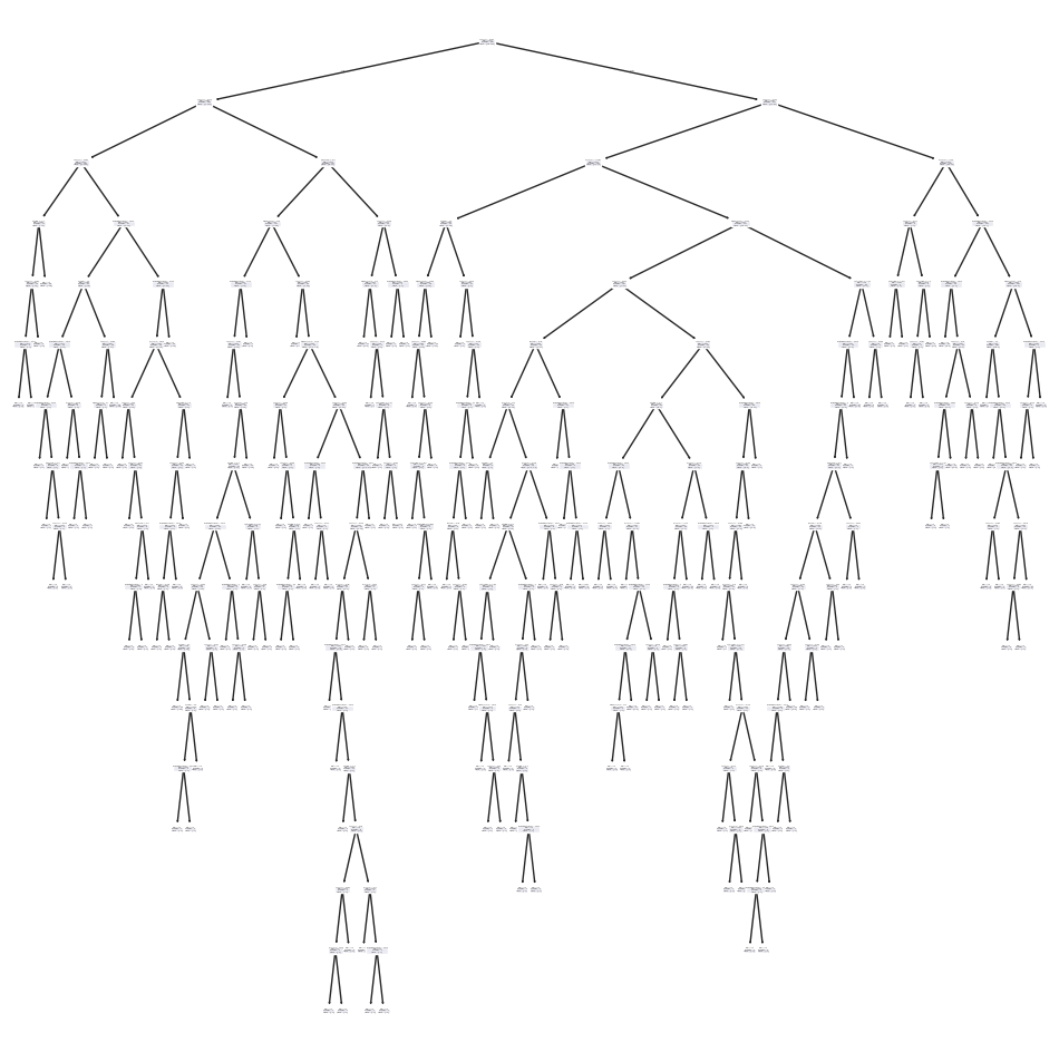
A lot of terminal nodes…

tree.get_n_leaves()

164

164 to be specific.

(d)

print(export_text(tree, feature_names=feature_names))

|--- LoyalCH <= 0.45
|   |--- LoyalCH <= 0.28
|   |   |--- LoyalCH <= 0.05
|   |   |   |--- StoreID <= 2.50
|   |   |   |   |--- LoyalCH <= 0.00
|   |   |   |   |   |--- WeekofPurchase <= 269.50
|   |   |   |   |   |   |--- class: CH
|   |   |   |   |   |--- WeekofPurchase >  269.50
|   |   |   |   |   |   |--- class: MM
|   |   |   |   |--- LoyalCH >  0.00
|   |   |   |   |   |--- class: MM
|   |   |   |--- StoreID >  2.50
|   |   |   |   |--- class: MM
|   |   |--- LoyalCH >  0.05
|   |   |   |--- WeekofPurchase <= 249.50
|   |   |   |   |--- STORE <= 1.50
|   |   |   |   |   |--- WeekofPurchase <= 235.50
|   |   |   |   |   |   |--- WeekofPurchase <= 232.00
|   |   |   |   |   |   |   |--- class: MM
|   |   |   |   |   |   |--- WeekofPurchase >  232.00
|   |   |   |   |   |   |   |--- SpecialCH <= 0.50
|   |   |   |   |   |   |   |   |--- class: CH
|   |   |   |   |   |   |   |--- SpecialCH >  0.50
|   |   |   |   |   |   |   |   |--- LoyalCH <= 0.22
|   |   |   |   |   |   |   |   |   |--- class: CH
|   |   |   |   |   |   |   |   |--- LoyalCH >  0.22
|   |   |   |   |   |   |   |   |   |--- class: MM
|   |   |   |   |   |--- WeekofPurchase >  235.50
|   |   |   |   |   |   |--- PriceDiff <= 0.13
|   |   |   |   |   |   |   |--- class: MM
|   |   |   |   |   |   |--- PriceDiff >  0.13
|   |   |   |   |   |   |   |--- WeekofPurchase <= 237.50
|   |   |   |   |   |   |   |   |--- class: MM
|   |   |   |   |   |   |   |--- WeekofPurchase >  237.50
|   |   |   |   |   |   |   |   |--- class: CH
|   |   |   |   |--- STORE >  1.50
|   |   |   |   |   |--- LoyalCH <= 0.07
|   |   |   |   |   |   |--- SalePriceCH <= 1.77
|   |   |   |   |   |   |   |--- class: MM
|   |   |   |   |   |   |--- SalePriceCH >  1.77
|   |   |   |   |   |   |   |--- class: CH
|   |   |   |   |   |--- LoyalCH >  0.07
|   |   |   |   |   |   |--- class: MM
|   |   |   |--- WeekofPurchase >  249.50
|   |   |   |   |--- WeekofPurchase <= 273.50
|   |   |   |   |   |--- PriceCH <= 1.88
|   |   |   |   |   |   |--- LoyalCH <= 0.18
|   |   |   |   |   |   |   |--- class: MM
|   |   |   |   |   |   |--- LoyalCH >  0.18
|   |   |   |   |   |   |   |--- LoyalCH <= 0.20
|   |   |   |   |   |   |   |   |--- class: CH
|   |   |   |   |   |   |   |--- LoyalCH >  0.20
|   |   |   |   |   |   |   |   |--- SpecialCH <= 0.50
|   |   |   |   |   |   |   |   |   |--- WeekofPurchase <= 272.50
|   |   |   |   |   |   |   |   |   |   |--- class: MM
|   |   |   |   |   |   |   |   |   |--- WeekofPurchase >  272.50
|   |   |   |   |   |   |   |   |   |   |--- class: CH
|   |   |   |   |   |   |   |   |--- SpecialCH >  0.50
|   |   |   |   |   |   |   |   |   |--- class: CH
|   |   |   |   |   |--- PriceCH >  1.88
|   |   |   |   |   |   |--- SpecialMM <= 0.50
|   |   |   |   |   |   |   |--- LoyalCH <= 0.17
|   |   |   |   |   |   |   |   |--- WeekofPurchase <= 261.00
|   |   |   |   |   |   |   |   |   |--- DiscCH <= 0.06
|   |   |   |   |   |   |   |   |   |   |--- class: MM
|   |   |   |   |   |   |   |   |   |--- DiscCH >  0.06
|   |   |   |   |   |   |   |   |   |   |--- class: CH
|   |   |   |   |   |   |   |   |--- WeekofPurchase >  261.00
|   |   |   |   |   |   |   |   |   |--- class: CH
|   |   |   |   |   |   |   |--- LoyalCH >  0.17
|   |   |   |   |   |   |   |   |--- class: CH
|   |   |   |   |   |   |--- SpecialMM >  0.50
|   |   |   |   |   |   |   |--- class: MM
|   |   |   |   |--- WeekofPurchase >  273.50
|   |   |   |   |   |--- class: MM
|   |--- LoyalCH >  0.28
|   |   |--- SpecialCH <= 0.50
|   |   |   |--- SalePriceMM <= 2.04
|   |   |   |   |--- WeekofPurchase <= 276.50
|   |   |   |   |   |--- LoyalCH <= 0.28
|   |   |   |   |   |   |--- class: CH
|   |   |   |   |   |--- LoyalCH >  0.28
|   |   |   |   |   |   |--- PriceMM <= 2.04
|   |   |   |   |   |   |   |--- StoreID <= 5.50
|   |   |   |   |   |   |   |   |--- WeekofPurchase <= 264.00
|   |   |   |   |   |   |   |   |   |--- LoyalCH <= 0.43
|   |   |   |   |   |   |   |   |   |   |--- STORE <= 2.50
|   |   |   |   |   |   |   |   |   |   |   |--- class: MM
|   |   |   |   |   |   |   |   |   |   |--- STORE >  2.50
|   |   |   |   |   |   |   |   |   |   |   |--- truncated branch of depth 3
|   |   |   |   |   |   |   |   |   |--- LoyalCH >  0.43
|   |   |   |   |   |   |   |   |   |   |--- LoyalCH <= 0.44
|   |   |   |   |   |   |   |   |   |   |   |--- class: CH
|   |   |   |   |   |   |   |   |   |   |--- LoyalCH >  0.44
|   |   |   |   |   |   |   |   |   |   |   |--- class: MM
|   |   |   |   |   |   |   |   |--- WeekofPurchase >  264.00
|   |   |   |   |   |   |   |   |   |--- WeekofPurchase <= 265.50
|   |   |   |   |   |   |   |   |   |   |--- class: CH
|   |   |   |   |   |   |   |   |   |--- WeekofPurchase >  265.50
|   |   |   |   |   |   |   |   |   |   |--- LoyalCH <= 0.41
|   |   |   |   |   |   |   |   |   |   |   |--- class: MM
|   |   |   |   |   |   |   |   |   |   |--- LoyalCH >  0.41
|   |   |   |   |   |   |   |   |   |   |   |--- class: CH
|   |   |   |   |   |   |   |--- StoreID >  5.50
|   |   |   |   |   |   |   |   |--- ListPriceDiff <= 0.12
|   |   |   |   |   |   |   |   |   |--- class: CH
|   |   |   |   |   |   |   |   |--- ListPriceDiff >  0.12
|   |   |   |   |   |   |   |   |   |--- LoyalCH <= 0.36
|   |   |   |   |   |   |   |   |   |   |--- class: CH
|   |   |   |   |   |   |   |   |   |--- LoyalCH >  0.36
|   |   |   |   |   |   |   |   |   |   |--- class: MM
|   |   |   |   |   |   |--- PriceMM >  2.04
|   |   |   |   |   |   |   |--- class: MM
|   |   |   |   |--- WeekofPurchase >  276.50
|   |   |   |   |   |--- class: CH
|   |   |   |--- SalePriceMM >  2.04
|   |   |   |   |--- LoyalCH <= 0.30
|   |   |   |   |   |--- class: CH
|   |   |   |   |--- LoyalCH >  0.30
|   |   |   |   |   |--- SalePriceCH <= 1.77
|   |   |   |   |   |   |--- LoyalCH <= 0.33
|   |   |   |   |   |   |   |--- class: CH
|   |   |   |   |   |   |--- LoyalCH >  0.33
|   |   |   |   |   |   |   |--- LoyalCH <= 0.35
|   |   |   |   |   |   |   |   |--- class: MM
|   |   |   |   |   |   |   |--- LoyalCH >  0.35
|   |   |   |   |   |   |   |   |--- StoreID <= 4.50
|   |   |   |   |   |   |   |   |   |--- WeekofPurchase <= 252.00
|   |   |   |   |   |   |   |   |   |   |--- class: CH
|   |   |   |   |   |   |   |   |   |--- WeekofPurchase >  252.00
|   |   |   |   |   |   |   |   |   |   |--- class: MM
|   |   |   |   |   |   |   |   |--- StoreID >  4.50
|   |   |   |   |   |   |   |   |   |--- class: CH
|   |   |   |   |   |--- SalePriceCH >  1.77
|   |   |   |   |   |   |--- LoyalCH <= 0.33
|   |   |   |   |   |   |   |--- WeekofPurchase <= 269.50
|   |   |   |   |   |   |   |   |--- class: MM
|   |   |   |   |   |   |   |--- WeekofPurchase >  269.50
|   |   |   |   |   |   |   |   |--- LoyalCH <= 0.31
|   |   |   |   |   |   |   |   |   |--- class: CH
|   |   |   |   |   |   |   |   |--- LoyalCH >  0.31
|   |   |   |   |   |   |   |   |   |--- class: MM
|   |   |   |   |   |   |--- LoyalCH >  0.33
|   |   |   |   |   |   |   |--- WeekofPurchase <= 269.00
|   |   |   |   |   |   |   |   |--- LoyalCH <= 0.42
|   |   |   |   |   |   |   |   |   |--- PriceDiff <= 0.38
|   |   |   |   |   |   |   |   |   |   |--- WeekofPurchase <= 243.00
|   |   |   |   |   |   |   |   |   |   |   |--- class: CH
|   |   |   |   |   |   |   |   |   |   |--- WeekofPurchase >  243.00
|   |   |   |   |   |   |   |   |   |   |   |--- truncated branch of depth 6
|   |   |   |   |   |   |   |   |   |--- PriceDiff >  0.38
|   |   |   |   |   |   |   |   |   |   |--- class: MM
|   |   |   |   |   |   |   |   |--- LoyalCH >  0.42
|   |   |   |   |   |   |   |   |   |--- PriceCH <= 1.93
|   |   |   |   |   |   |   |   |   |   |--- class: MM
|   |   |   |   |   |   |   |   |   |--- PriceCH >  1.93
|   |   |   |   |   |   |   |   |   |   |--- class: CH
|   |   |   |   |   |   |   |--- WeekofPurchase >  269.00
|   |   |   |   |   |   |   |   |--- class: MM
|   |   |--- SpecialCH >  0.50
|   |   |   |--- LoyalCH <= 0.41
|   |   |   |   |--- SalePriceCH <= 1.72
|   |   |   |   |   |--- class: CH
|   |   |   |   |--- SalePriceCH >  1.72
|   |   |   |   |   |--- LoyalCH <= 0.37
|   |   |   |   |   |   |--- class: MM
|   |   |   |   |   |--- LoyalCH >  0.37
|   |   |   |   |   |   |--- ListPriceDiff <= 0.17
|   |   |   |   |   |   |   |--- class: CH
|   |   |   |   |   |   |--- ListPriceDiff >  0.17
|   |   |   |   |   |   |   |--- LoyalCH <= 0.39
|   |   |   |   |   |   |   |   |--- class: CH
|   |   |   |   |   |   |   |--- LoyalCH >  0.39
|   |   |   |   |   |   |   |   |--- class: MM
|   |   |   |--- LoyalCH >  0.41
|   |   |   |   |--- WeekofPurchase <= 248.50
|   |   |   |   |   |--- class: CH
|   |   |   |   |--- WeekofPurchase >  248.50
|   |   |   |   |   |--- class: MM
|--- LoyalCH >  0.45
|   |--- LoyalCH <= 0.75
|   |   |--- PriceDiff <= -0.16
|   |   |   |--- STORE <= 2.50
|   |   |   |   |--- SalePriceMM <= 1.54
|   |   |   |   |   |--- LoyalCH <= 0.59
|   |   |   |   |   |   |--- class: MM
|   |   |   |   |   |--- LoyalCH >  0.59
|   |   |   |   |   |   |--- LoyalCH <= 0.71
|   |   |   |   |   |   |   |--- PctDiscMM <= 0.36
|   |   |   |   |   |   |   |   |--- class: CH
|   |   |   |   |   |   |   |--- PctDiscMM >  0.36
|   |   |   |   |   |   |   |   |--- PctDiscMM <= 0.38
|   |   |   |   |   |   |   |   |   |--- LoyalCH <= 0.67
|   |   |   |   |   |   |   |   |   |   |--- class: CH
|   |   |   |   |   |   |   |   |   |--- LoyalCH >  0.67
|   |   |   |   |   |   |   |   |   |   |--- class: MM
|   |   |   |   |   |   |   |   |--- PctDiscMM >  0.38
|   |   |   |   |   |   |   |   |   |--- class: MM
|   |   |   |   |   |   |--- LoyalCH >  0.71
|   |   |   |   |   |   |   |--- class: MM
|   |   |   |   |--- SalePriceMM >  1.54
|   |   |   |   |   |--- class: MM
|   |   |   |--- STORE >  2.50
|   |   |   |   |--- LoyalCH <= 0.52
|   |   |   |   |   |--- class: MM
|   |   |   |   |--- LoyalCH >  0.52
|   |   |   |   |   |--- LoyalCH <= 0.75
|   |   |   |   |   |   |--- WeekofPurchase <= 273.50
|   |   |   |   |   |   |   |--- WeekofPurchase <= 272.50
|   |   |   |   |   |   |   |   |--- DiscCH <= 0.05
|   |   |   |   |   |   |   |   |   |--- class: CH
|   |   |   |   |   |   |   |   |--- DiscCH >  0.05
|   |   |   |   |   |   |   |   |   |--- LoyalCH <= 0.68
|   |   |   |   |   |   |   |   |   |   |--- class: MM
|   |   |   |   |   |   |   |   |   |--- LoyalCH >  0.68
|   |   |   |   |   |   |   |   |   |   |--- class: CH
|   |   |   |   |   |   |   |--- WeekofPurchase >  272.50
|   |   |   |   |   |   |   |   |--- class: MM
|   |   |   |   |   |   |--- WeekofPurchase >  273.50
|   |   |   |   |   |   |   |--- class: CH
|   |   |   |   |   |--- LoyalCH >  0.75
|   |   |   |   |   |   |--- class: MM
|   |   |--- PriceDiff >  -0.16
|   |   |   |--- SalePriceMM <= 2.12
|   |   |   |   |--- LoyalCH <= 0.50
|   |   |   |   |   |--- DiscCH <= 0.05
|   |   |   |   |   |   |--- PriceCH <= 1.72
|   |   |   |   |   |   |   |--- STORE <= 1.50
|   |   |   |   |   |   |   |   |--- class: MM
|   |   |   |   |   |   |   |--- STORE >  1.50
|   |   |   |   |   |   |   |   |--- class: CH
|   |   |   |   |   |   |--- PriceCH >  1.72
|   |   |   |   |   |   |   |--- PriceDiff <= 0.23
|   |   |   |   |   |   |   |   |--- StoreID <= 3.50
|   |   |   |   |   |   |   |   |   |--- ListPriceDiff <= 0.28
|   |   |   |   |   |   |   |   |   |   |--- WeekofPurchase <= 245.50
|   |   |   |   |   |   |   |   |   |   |   |--- class: MM
|   |   |   |   |   |   |   |   |   |   |--- WeekofPurchase >  245.50
|   |   |   |   |   |   |   |   |   |   |   |--- truncated branch of depth 3
|   |   |   |   |   |   |   |   |   |--- ListPriceDiff >  0.28
|   |   |   |   |   |   |   |   |   |   |--- class: CH
|   |   |   |   |   |   |   |   |--- StoreID >  3.50
|   |   |   |   |   |   |   |   |   |--- WeekofPurchase <= 255.50
|   |   |   |   |   |   |   |   |   |   |--- PriceMM <= 2.04
|   |   |   |   |   |   |   |   |   |   |   |--- truncated branch of depth 4
|   |   |   |   |   |   |   |   |   |   |--- PriceMM >  2.04
|   |   |   |   |   |   |   |   |   |   |   |--- class: CH
|   |   |   |   |   |   |   |   |   |--- WeekofPurchase >  255.50
|   |   |   |   |   |   |   |   |   |   |--- class: MM
|   |   |   |   |   |   |   |--- PriceDiff >  0.23
|   |   |   |   |   |   |   |   |--- WeekofPurchase <= 252.00
|   |   |   |   |   |   |   |   |   |--- class: CH
|   |   |   |   |   |   |   |   |--- WeekofPurchase >  252.00
|   |   |   |   |   |   |   |   |   |--- LoyalCH <= 0.48
|   |   |   |   |   |   |   |   |   |   |--- class: MM
|   |   |   |   |   |   |   |   |   |--- LoyalCH >  0.48
|   |   |   |   |   |   |   |   |   |   |--- class: CH
|   |   |   |   |   |--- DiscCH >  0.05
|   |   |   |   |   |   |--- WeekofPurchase <= 252.50
|   |   |   |   |   |   |   |--- class: CH
|   |   |   |   |   |   |--- WeekofPurchase >  252.50
|   |   |   |   |   |   |   |--- WeekofPurchase <= 261.00
|   |   |   |   |   |   |   |   |--- class: MM
|   |   |   |   |   |   |   |--- WeekofPurchase >  261.00
|   |   |   |   |   |   |   |   |--- WeekofPurchase <= 271.50
|   |   |   |   |   |   |   |   |   |--- class: CH
|   |   |   |   |   |   |   |   |--- WeekofPurchase >  271.50
|   |   |   |   |   |   |   |   |   |--- class: CH
|   |   |   |   |--- LoyalCH >  0.50
|   |   |   |   |   |--- LoyalCH <= 0.65
|   |   |   |   |   |   |--- StoreID <= 2.50
|   |   |   |   |   |   |   |--- WeekofPurchase <= 233.50
|   |   |   |   |   |   |   |   |--- LoyalCH <= 0.59
|   |   |   |   |   |   |   |   |   |--- class: MM
|   |   |   |   |   |   |   |   |--- LoyalCH >  0.59
|   |   |   |   |   |   |   |   |   |--- class: CH
|   |   |   |   |   |   |   |--- WeekofPurchase >  233.50
|   |   |   |   |   |   |   |   |--- PriceDiff <= -0.06
|   |   |   |   |   |   |   |   |   |--- class: MM
|   |   |   |   |   |   |   |   |--- PriceDiff >  -0.06
|   |   |   |   |   |   |   |   |   |--- WeekofPurchase <= 272.50
|   |   |   |   |   |   |   |   |   |   |--- WeekofPurchase <= 236.50
|   |   |   |   |   |   |   |   |   |   |   |--- truncated branch of depth 2
|   |   |   |   |   |   |   |   |   |   |--- WeekofPurchase >  236.50
|   |   |   |   |   |   |   |   |   |   |   |--- class: CH
|   |   |   |   |   |   |   |   |   |--- WeekofPurchase >  272.50
|   |   |   |   |   |   |   |   |   |   |--- LoyalCH <= 0.58
|   |   |   |   |   |   |   |   |   |   |   |--- class: CH
|   |   |   |   |   |   |   |   |   |   |--- LoyalCH >  0.58
|   |   |   |   |   |   |   |   |   |   |   |--- class: MM
|   |   |   |   |   |   |--- StoreID >  2.50
|   |   |   |   |   |   |   |--- PriceDiff <= 0.32
|   |   |   |   |   |   |   |   |--- PriceDiff <= -0.13
|   |   |   |   |   |   |   |   |   |--- WeekofPurchase <= 233.50
|   |   |   |   |   |   |   |   |   |   |--- class: CH
|   |   |   |   |   |   |   |   |   |--- WeekofPurchase >  233.50
|   |   |   |   |   |   |   |   |   |   |--- LoyalCH <= 0.58
|   |   |   |   |   |   |   |   |   |   |   |--- class: CH
|   |   |   |   |   |   |   |   |   |   |--- LoyalCH >  0.58
|   |   |   |   |   |   |   |   |   |   |   |--- class: MM
|   |   |   |   |   |   |   |   |--- PriceDiff >  -0.13
|   |   |   |   |   |   |   |   |   |--- class: CH
|   |   |   |   |   |   |   |--- PriceDiff >  0.32
|   |   |   |   |   |   |   |   |--- WeekofPurchase <= 251.50
|   |   |   |   |   |   |   |   |   |--- class: MM
|   |   |   |   |   |   |   |   |--- WeekofPurchase >  251.50
|   |   |   |   |   |   |   |   |   |--- class: CH
|   |   |   |   |   |--- LoyalCH >  0.65
|   |   |   |   |   |   |--- WeekofPurchase <= 266.50
|   |   |   |   |   |   |   |--- LoyalCH <= 0.71
|   |   |   |   |   |   |   |   |--- LoyalCH <= 0.69
|   |   |   |   |   |   |   |   |   |--- PriceMM <= 1.74
|   |   |   |   |   |   |   |   |   |   |--- class: MM
|   |   |   |   |   |   |   |   |   |--- PriceMM >  1.74
|   |   |   |   |   |   |   |   |   |   |--- ListPriceDiff <= 0.16
|   |   |   |   |   |   |   |   |   |   |   |--- class: CH
|   |   |   |   |   |   |   |   |   |   |--- ListPriceDiff >  0.16
|   |   |   |   |   |   |   |   |   |   |   |--- truncated branch of depth 5
|   |   |   |   |   |   |   |   |--- LoyalCH >  0.69
|   |   |   |   |   |   |   |   |   |--- class: MM
|   |   |   |   |   |   |   |--- LoyalCH >  0.71
|   |   |   |   |   |   |   |   |--- class: CH
|   |   |   |   |   |   |--- WeekofPurchase >  266.50
|   |   |   |   |   |   |   |--- class: MM
|   |   |   |--- SalePriceMM >  2.12
|   |   |   |   |--- ListPriceDiff <= 0.43
|   |   |   |   |   |--- WeekofPurchase <= 261.50
|   |   |   |   |   |   |--- WeekofPurchase <= 260.00
|   |   |   |   |   |   |   |--- SpecialCH <= 0.50
|   |   |   |   |   |   |   |   |--- DiscCH <= 0.06
|   |   |   |   |   |   |   |   |   |--- LoyalCH <= 0.74
|   |   |   |   |   |   |   |   |   |   |--- LoyalCH <= 0.51
|   |   |   |   |   |   |   |   |   |   |   |--- truncated branch of depth 3
|   |   |   |   |   |   |   |   |   |   |--- LoyalCH >  0.51
|   |   |   |   |   |   |   |   |   |   |   |--- class: CH
|   |   |   |   |   |   |   |   |   |--- LoyalCH >  0.74
|   |   |   |   |   |   |   |   |   |   |--- LoyalCH <= 0.74
|   |   |   |   |   |   |   |   |   |   |   |--- class: MM
|   |   |   |   |   |   |   |   |   |   |--- LoyalCH >  0.74
|   |   |   |   |   |   |   |   |   |   |   |--- class: CH
|   |   |   |   |   |   |   |   |--- DiscCH >  0.06
|   |   |   |   |   |   |   |   |   |--- LoyalCH <= 0.59
|   |   |   |   |   |   |   |   |   |   |--- class: MM
|   |   |   |   |   |   |   |   |   |--- LoyalCH >  0.59
|   |   |   |   |   |   |   |   |   |   |--- class: CH
|   |   |   |   |   |   |   |--- SpecialCH >  0.50
|   |   |   |   |   |   |   |   |--- LoyalCH <= 0.59
|   |   |   |   |   |   |   |   |   |--- class: CH
|   |   |   |   |   |   |   |   |--- LoyalCH >  0.59
|   |   |   |   |   |   |   |   |   |--- class: MM
|   |   |   |   |   |   |--- WeekofPurchase >  260.00
|   |   |   |   |   |   |   |--- class: MM
|   |   |   |   |   |--- WeekofPurchase >  261.50
|   |   |   |   |   |   |--- class: CH
|   |   |   |   |--- ListPriceDiff >  0.43
|   |   |   |   |   |--- LoyalCH <= 0.57
|   |   |   |   |   |   |--- class: MM
|   |   |   |   |   |--- LoyalCH >  0.57
|   |   |   |   |   |   |--- class: CH
|   |--- LoyalCH >  0.75
|   |   |--- PriceDiff <= -0.39
|   |   |   |--- LoyalCH <= 0.98
|   |   |   |   |--- PctDiscMM <= 0.22
|   |   |   |   |   |--- class: CH
|   |   |   |   |--- PctDiscMM >  0.22
|   |   |   |   |   |--- class: MM
|   |   |   |--- LoyalCH >  0.98
|   |   |   |   |--- SpecialMM <= 0.50
|   |   |   |   |   |--- LoyalCH <= 1.00
|   |   |   |   |   |   |--- class: MM
|   |   |   |   |   |--- LoyalCH >  1.00
|   |   |   |   |   |   |--- class: CH
|   |   |   |   |--- SpecialMM >  0.50
|   |   |   |   |   |--- class: CH
|   |   |--- PriceDiff >  -0.39
|   |   |   |--- WeekofPurchase <= 241.50
|   |   |   |   |--- WeekofPurchase <= 236.50
|   |   |   |   |   |--- class: CH
|   |   |   |   |--- WeekofPurchase >  236.50
|   |   |   |   |   |--- LoyalCH <= 0.93
|   |   |   |   |   |   |--- WeekofPurchase <= 238.50
|   |   |   |   |   |   |   |--- ListPriceDiff <= 0.27
|   |   |   |   |   |   |   |   |--- class: CH
|   |   |   |   |   |   |   |--- ListPriceDiff >  0.27
|   |   |   |   |   |   |   |   |--- class: MM
|   |   |   |   |   |   |--- WeekofPurchase >  238.50
|   |   |   |   |   |   |   |--- class: CH
|   |   |   |   |   |--- LoyalCH >  0.93
|   |   |   |   |   |   |--- LoyalCH <= 0.98
|   |   |   |   |   |   |   |--- class: MM
|   |   |   |   |   |   |--- LoyalCH >  0.98
|   |   |   |   |   |   |   |--- class: CH
|   |   |   |--- WeekofPurchase >  241.50
|   |   |   |   |--- SalePriceMM <= 2.26
|   |   |   |   |   |--- STORE <= 1.50
|   |   |   |   |   |   |--- class: CH
|   |   |   |   |   |--- STORE >  1.50
|   |   |   |   |   |   |--- WeekofPurchase <= 263.50
|   |   |   |   |   |   |   |--- class: CH
|   |   |   |   |   |   |--- WeekofPurchase >  263.50
|   |   |   |   |   |   |   |--- WeekofPurchase <= 264.50
|   |   |   |   |   |   |   |   |--- LoyalCH <= 0.96
|   |   |   |   |   |   |   |   |   |--- class: CH
|   |   |   |   |   |   |   |   |--- LoyalCH >  0.96
|   |   |   |   |   |   |   |   |   |--- class: MM
|   |   |   |   |   |   |   |--- WeekofPurchase >  264.50
|   |   |   |   |   |   |   |   |--- LoyalCH <= 0.88
|   |   |   |   |   |   |   |   |   |--- LoyalCH <= 0.87
|   |   |   |   |   |   |   |   |   |   |--- class: CH
|   |   |   |   |   |   |   |   |   |--- LoyalCH >  0.87
|   |   |   |   |   |   |   |   |   |   |--- class: MM
|   |   |   |   |   |   |   |   |--- LoyalCH >  0.88
|   |   |   |   |   |   |   |   |   |--- class: CH
|   |   |   |   |--- SalePriceMM >  2.26
|   |   |   |   |   |--- WeekofPurchase <= 254.50
|   |   |   |   |   |   |--- LoyalCH <= 0.92
|   |   |   |   |   |   |   |--- class: MM
|   |   |   |   |   |   |--- LoyalCH >  0.92
|   |   |   |   |   |   |   |--- class: CH
|   |   |   |   |   |--- WeekofPurchase >  254.50
|   |   |   |   |   |   |--- class: CH

I’m choosing the first terminal node since it’s the easiest to parse.

|--- LoyalCH <= 0.45
|   |--- LoyalCH <= 0.28
|   |   |--- LoyalCH <= 0.05
|   |   |   |--- StoreID <= 2.50
|   |   |   |   |--- LoyalCH <= 0.00
|   |   |   |   |   |--- WeekofPurchase <= 269.50
|   |   |   |   |   |   |--- class: CH

We go to the variable LoyalCH if it’s less than or equal to \(0.45\) we go left, we do this to more times with values \(0.28\), \(0.05\), then we check if StoreID is less than or equal to \(2.50\) if it is we go left, then if LoyalCH is less than or equal to \(0\) we go left and finally if WeekofPurchase is less than or equal to \(269.5\) we go left and classify the observation as CH.

(e)

y_pred = results.predict(X_test)
confusion_table(y_pred, y_test)

Truth	CH	MM
Predicted
CH	132	40
MM	25	73

The test error rate is:

1 - accuracy_score(y_test, y_pred)

0.2407407407407407

(f)

kfold = skm.KFold(5,
                  shuffle=True,
                  random_state=6)

grid = skm.GridSearchCV(tree,
                        {'max_depth': np.arange(1, 100)},
                        refit=True,
                        cv=kfold,
                        scoring='accuracy')

grid = grid.fit(X_train, y_train)
grid.best_params_

{'max_depth': 3}

The optimal tree size is \(3\).

best_tree = grid.best_estimator_
y_pred = best_tree.predict(X_test)
confusion_table(y_pred, y_test)

Truth	CH	MM
Predicted
CH	139	31
MM	18	82

(g)

x = grid.cv_results_['param_max_depth'].data # tree depth
y = 1 - grid.cv_results_['mean_test_score'] # classification error rate = 1 - accuracy

_, ax = plt.subplots()
sns.lineplot(x=x,
             y=y,
             ax=ax)

ax.plot(x[np.argmin(y)], y.min(), 'Dr', label=f'min cv error = {y.min():.4f}')
ax.set_xlabel('Max Depth')
ax.set_ylabel('CV Classification Error Rate')
ax.legend();

(h)

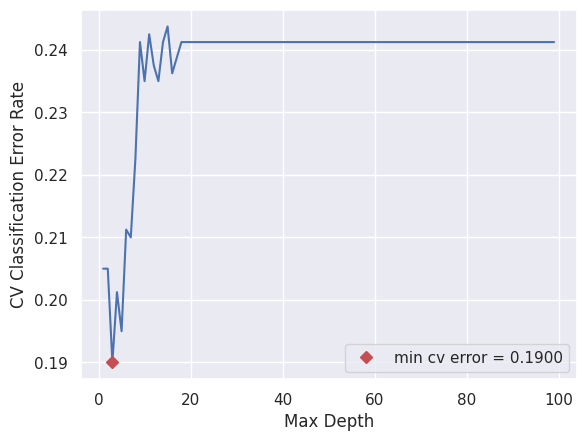
A tree of size 3 has the lowest cv classification error rate.

x[np.argmin(y)]

3

And \(8\) terminal nodes.

best_tree.get_n_leaves()

8

(i)

Now we’ll prune the tree of size 3 we obtained from cross validation.

ccp_path = best_tree.cost_complexity_pruning_path(X_train, y_train)

kfold = skm.KFold(5,
                  shuffle=True,
                  random_state=3)

grid = skm.GridSearchCV(best_tree,
                        {'ccp_alpha': ccp_path.ccp_alphas},
                        refit=True,
                        cv=kfold,
                        scoring='accuracy')

grid = grid.fit(X_train, y_train)
grid.best_params_, grid.best_estimator_.get_n_leaves()

({'ccp_alpha': 0.014143149663851926}, 4)

Cross validation leads to the selection of a pruned tree with \(4\) terminal nodes.

pruned_tree = grid.best_estimator_

(j) Training error rate:

For the unpruned tree with \(8\) terminal nodes.

1 - best_tree.score(X_train, y_train)

0.15249999999999997

For the pruned tree with \(4\) terminal nodes.

1 - pruned_tree.score(X_train, y_train)

0.16500000000000004

We can see that the training error rate for the pruned tree is higher.

(k) Test error rate:

For the unpruned tree with \(8\) terminal nodes.

y_pred = best_tree.predict(X_test)
1 - accuracy_score(y_test, y_pred)

0.18148148148148147

For the pruned tree with \(4\) terminal nodes.

y_pred = pruned_tree.predict(X_test)
1 - accuracy_score(y_test, y_pred)

0.18148148148148147

They’re exactly the same.

Q10.

hitters = load_data('Hitters')
hitters.head()

	AtBat	Hits	HmRun	Runs	RBI	Walks	Years	CAtBat	CHits	CHmRun	CRuns	CRBI	CWalks	League	Division	PutOuts	Assists	Errors	Salary	NewLeague
0	293	66	1	30	29	14	1	293	66	1	30	29	14	A	E	446	33	20	NaN	A
1	315	81	7	24	38	39	14	3449	835	69	321	414	375	N	W	632	43	10	475.0	N
2	479	130	18	66	72	76	3	1624	457	63	224	266	263	A	W	880	82	14	480.0	A
3	496	141	20	65	78	37	11	5628	1575	225	828	838	354	N	E	200	11	3	500.0	N
4	321	87	10	39	42	30	2	396	101	12	48	46	33	N	E	805	40	4	91.5	N

hitters.info()

<class 'pandas.core.frame.DataFrame'>
RangeIndex: 322 entries, 0 to 321
Data columns (total 20 columns):
 #   Column     Non-Null Count  Dtype   
---  ------     --------------  -----   
 0   AtBat      322 non-null    int64   
 1   Hits       322 non-null    int64   
 2   HmRun      322 non-null    int64   
 3   Runs       322 non-null    int64   
 4   RBI        322 non-null    int64   
 5   Walks      322 non-null    int64   
 6   Years      322 non-null    int64   
 7   CAtBat     322 non-null    int64   
 8   CHits      322 non-null    int64   
 9   CHmRun     322 non-null    int64   
 10  CRuns      322 non-null    int64   
 11  CRBI       322 non-null    int64   
 12  CWalks     322 non-null    int64   
 13  League     322 non-null    category
 14  Division   322 non-null    category
 15  PutOuts    322 non-null    int64   
 16  Assists    322 non-null    int64   
 17  Errors     322 non-null    int64   
 18  Salary     263 non-null    float64 
 19  NewLeague  322 non-null    category
dtypes: category(3), float64(1), int64(16)
memory usage: 44.2 KB

hitters.describe()

	AtBat	Hits	HmRun	Runs	RBI	Walks	Years	CAtBat	CHits	CHmRun	CRuns	CRBI	CWalks	PutOuts	Assists	Errors	Salary
count	322.000000	322.000000	322.000000	322.000000	322.000000	322.000000	322.000000	322.00000	322.000000	322.000000	322.000000	322.000000	322.000000	322.000000	322.000000	322.000000	263.000000
mean	380.928571	101.024845	10.770186	50.909938	48.027950	38.742236	7.444099	2648.68323	717.571429	69.490683	358.795031	330.118012	260.239130	288.937888	106.913043	8.040373	535.925882
std	153.404981	46.454741	8.709037	26.024095	26.166895	21.639327	4.926087	2324.20587	654.472627	86.266061	334.105886	333.219617	267.058085	280.704614	136.854876	6.368359	451.118681
min	16.000000	1.000000	0.000000	0.000000	0.000000	0.000000	1.000000	19.00000	4.000000	0.000000	1.000000	0.000000	0.000000	0.000000	0.000000	0.000000	67.500000
25%	255.250000	64.000000	4.000000	30.250000	28.000000	22.000000	4.000000	816.75000	209.000000	14.000000	100.250000	88.750000	67.250000	109.250000	7.000000	3.000000	190.000000
50%	379.500000	96.000000	8.000000	48.000000	44.000000	35.000000	6.000000	1928.00000	508.000000	37.500000	247.000000	220.500000	170.500000	212.000000	39.500000	6.000000	425.000000
75%	512.000000	137.000000	16.000000	69.000000	64.750000	53.000000	11.000000	3924.25000	1059.250000	90.000000	526.250000	426.250000	339.250000	325.000000	166.000000	11.000000	750.000000
max	687.000000	238.000000	40.000000	130.000000	121.000000	105.000000	24.000000	14053.00000	4256.000000	548.000000	2165.000000	1659.000000	1566.000000	1378.000000	492.000000	32.000000	2460.000000

hitters.describe(include='category')

	League	Division	NewLeague
count	322	322	322
unique	2	2	2
top	A	W	A
freq	175	165	176

(a)

hitters['Salary'].isna().sum()

59

59 null values in the Salary column, we’ll proceed by dropping them.

hitters.dropna(subset=['Salary'], inplace=True)
hitters['Salary'].isna().sum()

0

Now we’ll log-transform the salaries.

hitters['Salary'] = np.log(hitters['Salary'])
hitters['Salary'].describe()

count    263.000000
mean       5.927222
std        0.889192
min        4.212128
25%        5.247024
50%        6.052089
75%        6.620073
max        7.807917
Name: Salary, dtype: float64

(b)

model = MS(hitters.columns.drop('Salary'), intercept=False)
D = model.fit_transform(hitters)
feature_names = list(D.columns)
X = np.asarray(D)
y = hitters['Salary']

X_train, y_train = X[:200], y[:200]
X_test, y_test = X[200:], y[200:]

(c)

We’ll perform boosting with 1000 trees and a \(100\) values for the shrinkage paramater ranging from 0.0001 to 0.1.

lambdas = np.linspace(0.0001, 0.2, 100, endpoint=True)
train_errors = np.zeros_like(lambdas)
test_errors = np.zeros_like(lambdas)

min_error = np.infty
best_booster = None

for idx, lam in enumerate(lambdas):
    boost_hitters = GBR(n_estimators=1000,
                    learning_rate=lam,
                    max_depth=3,
                    random_state=1)
    boost_hitters.fit(X_train, y_train)
    
    train_errors[idx] = np.mean((y_train - boost_hitters.predict(X_train))**2)
    test_errors[idx] = np.mean((y_test - boost_hitters.predict(X_test))**2)
    
    if test_errors[idx] < min_error:
        best_booster = boost_hitters
        min_error = test_errors[idx]

x = lambdas
y = train_errors
_, ax = plt.subplots()
sns.lineplot(x=x,
             y=y,
             ax=ax)

ax.plot(x[np.argmin(y)], y.min(), 'Dr', label=f'min train error = {y.min():.4f}')
ax.set_xlabel('Shrinkage Parameter $\\lambda$')
ax.set_ylabel('Training MSE')
ax.legend();

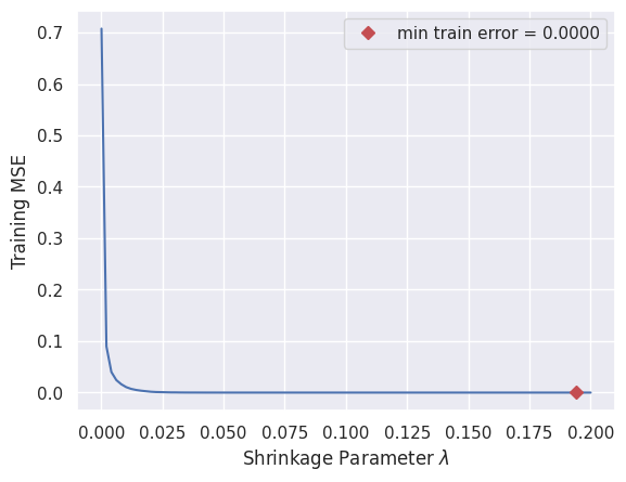
Shrinkage value that minimizes train MSE.

x[np.argmin(y)]

0.19394242424242425

(d)

x = lambdas
y = test_errors
_, ax = plt.subplots()
sns.lineplot(x=x,
             y=y,
             ax=ax)

ax.plot(x[np.argmin(y)], y.min(), 'Dr', label=f'min test error = {y.min():.4f}')
ax.set_xlabel('Shrinkage Parameter $\\lambda$')
ax.set_ylabel('Test MSE')
ax.legend();

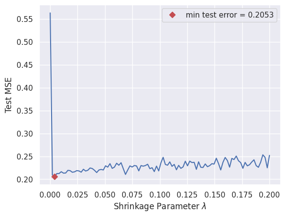
boost_MSE = test_errors.min()
boost_MSE

0.20530216513114846

Shrinkage value that minimizes test MSE.

x[np.argmin(y)]

0.004138383838383839

(e)

We’ll apply linear regression and the lasso methods to the data to see how they compare to boosting.

Linear regression test MSE:

lr = skl.LinearRegression().fit(X_train, y_train)
lr_MSE = np.mean((lr.predict(X_test) - y_test)**2)
lr_MSE

0.4917959375454946

kfold = skm.KFold(n_splits=5,
               shuffle=True,
               random_state=2)

scaler = StandardScaler()

lassoCV = skl.ElasticNetCV(l1_ratio=1,
                           cv=kfold,
                           max_iter=2000)

pipeCV = Pipeline([('scaler', scaler),
                ('lasso', lassoCV)])
pipeCV.fit(X_train, y_train)

Pipeline(steps=[('scaler', StandardScaler()),
                ('lasso',
                 ElasticNetCV(cv=KFold(n_splits=5, random_state=2, shuffle=True),
                              l1_ratio=1, max_iter=2000))])

In a Jupyter environment, please rerun this cell to show the HTML representation or trust the notebook.
On GitHub, the HTML representation is unable to render, please try loading this page with nbviewer.org.

Lasso test MSE:

lasso_MSE = np.mean((pipeCV.predict(X_test) - y_test)**2)
lasso_MSE

0.4710027646164625

Now we’ll compare their RMSE:

print(f"Boosting RMSE: {np.sqrt(boost_MSE):.4f}")
print(f"Linear Regression RMSE: {np.sqrt(lr_MSE):.4f}")
print(f"Lasso RMSE: {np.sqrt(lasso_MSE):.4f}")

Boosting RMSE: 0.4531
Linear Regression RMSE: 0.7013
Lasso RMSE: 0.6863

We can see that while their test RMSE is still within one standard deviation of the mean, linear regression and the lasso perform much worse on this data set than boosting does.

hitters['Salary'].std(), hitters['Salary'].mean()

(0.8891923883918419, 5.927221541221392)

(f)

feature_imp = pd.DataFrame(
    {'importance':best_booster.feature_importances_},
    index=feature_names)

plt.figure().set_size_inches(8, 6)
sns.barplot(feature_imp.sort_values(by='importance', ascending=True).T * 100/feature_imp['importance'].max(), orient='h');

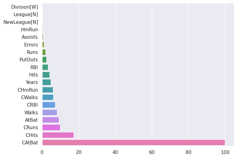
The CAtBat (Number of times at bat during his career) predictor seems to be the most important when predicting Salary for the boosted model.

To understand what the other predictors mean you can go to this page.

(g)

bagging_hitters = RF(n_estimators=500,
                    max_features=X_train.shape[1],
                    random_state=1).fit(X_train, y_train)
np.mean((bagging_hitters.predict(X_test) - y_test)**2)

0.2296193952740068

We got a test MSE of \(0.2296\) with bagging which is slightly higher than the best test MSE we got with boosting \(0.2053\).

Q11.

caravan = load_data('Caravan')
caravan.head()

	MOSTYPE	MAANTHUI	MGEMOMV	MGEMLEEF	MOSHOOFD	MGODRK	MGODPR	MGODOV	MGODGE	MRELGE	...	APERSONG	AGEZONG	AWAOREG	ABRAND	AZEILPL	APLEZIER	AFIETS	AINBOED	ABYSTAND	Purchase
0	33	1	3	2	8	0	5	1	3	7	...	0	0	0	1	0	0	0	0	0	No
1	37	1	2	2	8	1	4	1	4	6	...	0	0	0	1	0	0	0	0	0	No
2	37	1	2	2	8	0	4	2	4	3	...	0	0	0	1	0	0	0	0	0	No
3	9	1	3	3	3	2	3	2	4	5	...	0	0	0	1	0	0	0	0	0	No
4	40	1	4	2	10	1	4	1	4	7	...	0	0	0	1	0	0	0	0	0	No

5 rows × 86 columns

caravan.info()

<class 'pandas.core.frame.DataFrame'>
RangeIndex: 5822 entries, 0 to 5821
Data columns (total 86 columns):
 #   Column    Non-Null Count  Dtype   
---  ------    --------------  -----   
 0   MOSTYPE   5822 non-null   int64   
 1   MAANTHUI  5822 non-null   int64   
 2   MGEMOMV   5822 non-null   int64   
 3   MGEMLEEF  5822 non-null   int64   
 4   MOSHOOFD  5822 non-null   int64   
 5   MGODRK    5822 non-null   int64   
 6   MGODPR    5822 non-null   int64   
 7   MGODOV    5822 non-null   int64   
 8   MGODGE    5822 non-null   int64   
 9   MRELGE    5822 non-null   int64   
 10  MRELSA    5822 non-null   int64   
 11  MRELOV    5822 non-null   int64   
 12  MFALLEEN  5822 non-null   int64   
 13  MFGEKIND  5822 non-null   int64   
 14  MFWEKIND  5822 non-null   int64   
 15  MOPLHOOG  5822 non-null   int64   
 16  MOPLMIDD  5822 non-null   int64   
 17  MOPLLAAG  5822 non-null   int64   
 18  MBERHOOG  5822 non-null   int64   
 19  MBERZELF  5822 non-null   int64   
 20  MBERBOER  5822 non-null   int64   
 21  MBERMIDD  5822 non-null   int64   
 22  MBERARBG  5822 non-null   int64   
 23  MBERARBO  5822 non-null   int64   
 24  MSKA      5822 non-null   int64   
 25  MSKB1     5822 non-null   int64   
 26  MSKB2     5822 non-null   int64   
 27  MSKC      5822 non-null   int64   
 28  MSKD      5822 non-null   int64   
 29  MHHUUR    5822 non-null   int64   
 30  MHKOOP    5822 non-null   int64   
 31  MAUT1     5822 non-null   int64   
 32  MAUT2     5822 non-null   int64   
 33  MAUT0     5822 non-null   int64   
 34  MZFONDS   5822 non-null   int64   
 35  MZPART    5822 non-null   int64   
 36  MINKM30   5822 non-null   int64   
 37  MINK3045  5822 non-null   int64   
 38  MINK4575  5822 non-null   int64   
 39  MINK7512  5822 non-null   int64   
 40  MINK123M  5822 non-null   int64   
 41  MINKGEM   5822 non-null   int64   
 42  MKOOPKLA  5822 non-null   int64   
 43  PWAPART   5822 non-null   int64   
 44  PWABEDR   5822 non-null   int64   
 45  PWALAND   5822 non-null   int64   
 46  PPERSAUT  5822 non-null   int64   
 47  PBESAUT   5822 non-null   int64   
 48  PMOTSCO   5822 non-null   int64   
 49  PVRAAUT   5822 non-null   int64   
 50  PAANHANG  5822 non-null   int64   
 51  PTRACTOR  5822 non-null   int64   
 52  PWERKT    5822 non-null   int64   
 53  PBROM     5822 non-null   int64   
 54  PLEVEN    5822 non-null   int64   
 55  PPERSONG  5822 non-null   int64   
 56  PGEZONG   5822 non-null   int64   
 57  PWAOREG   5822 non-null   int64   
 58  PBRAND    5822 non-null   int64   
 59  PZEILPL   5822 non-null   int64   
 60  PPLEZIER  5822 non-null   int64   
 61  PFIETS    5822 non-null   int64   
 62  PINBOED   5822 non-null   int64   
 63  PBYSTAND  5822 non-null   int64   
 64  AWAPART   5822 non-null   int64   
 65  AWABEDR   5822 non-null   int64   
 66  AWALAND   5822 non-null   int64   
 67  APERSAUT  5822 non-null   int64   
 68  ABESAUT   5822 non-null   int64   
 69  AMOTSCO   5822 non-null   int64   
 70  AVRAAUT   5822 non-null   int64   
 71  AAANHANG  5822 non-null   int64   
 72  ATRACTOR  5822 non-null   int64   
 73  AWERKT    5822 non-null   int64   
 74  ABROM     5822 non-null   int64   
 75  ALEVEN    5822 non-null   int64   
 76  APERSONG  5822 non-null   int64   
 77  AGEZONG   5822 non-null   int64   
 78  AWAOREG   5822 non-null   int64   
 79  ABRAND    5822 non-null   int64   
 80  AZEILPL   5822 non-null   int64   
 81  APLEZIER  5822 non-null   int64   
 82  AFIETS    5822 non-null   int64   
 83  AINBOED   5822 non-null   int64   
 84  ABYSTAND  5822 non-null   int64   
 85  Purchase  5822 non-null   category
dtypes: category(1), int64(85)
memory usage: 3.8 MB

caravan.describe()

	MOSTYPE	MAANTHUI	MGEMOMV	MGEMLEEF	MOSHOOFD	MGODRK	MGODPR	MGODOV	MGODGE	MRELGE	...	ALEVEN	APERSONG	AGEZONG	AWAOREG	ABRAND	AZEILPL	APLEZIER	AFIETS	AINBOED	ABYSTAND
count	5822.000000	5822.000000	5822.000000	5822.000000	5822.000000	5822.000000	5822.000000	5822.000000	5822.000000	5822.000000	...	5822.000000	5822.000000	5822.000000	5822.000000	5822.000000	5822.000000	5822.000000	5822.000000	5822.000000	5822.000000
mean	24.253349	1.110615	2.678805	2.991240	5.773617	0.696496	4.626932	1.069907	3.258502	6.183442	...	0.076606	0.005325	0.006527	0.004638	0.570079	0.000515	0.006012	0.031776	0.007901	0.014256
std	12.846706	0.405842	0.789835	0.814589	2.856760	1.003234	1.715843	1.017503	1.597647	1.909482	...	0.377569	0.072782	0.080532	0.077403	0.562058	0.022696	0.081632	0.210986	0.090463	0.119996
min	1.000000	1.000000	1.000000	1.000000	1.000000	0.000000	0.000000	0.000000	0.000000	0.000000	...	0.000000	0.000000	0.000000	0.000000	0.000000	0.000000	0.000000	0.000000	0.000000	0.000000
25%	10.000000	1.000000	2.000000	2.000000	3.000000	0.000000	4.000000	0.000000	2.000000	5.000000	...	0.000000	0.000000	0.000000	0.000000	0.000000	0.000000	0.000000	0.000000	0.000000	0.000000
50%	30.000000	1.000000	3.000000	3.000000	7.000000	0.000000	5.000000	1.000000	3.000000	6.000000	...	0.000000	0.000000	0.000000	0.000000	1.000000	0.000000	0.000000	0.000000	0.000000	0.000000
75%	35.000000	1.000000	3.000000	3.000000	8.000000	1.000000	6.000000	2.000000	4.000000	7.000000	...	0.000000	0.000000	0.000000	0.000000	1.000000	0.000000	0.000000	0.000000	0.000000	0.000000
max	41.000000	10.000000	5.000000	6.000000	10.000000	9.000000	9.000000	5.000000	9.000000	9.000000	...	8.000000	1.000000	1.000000	2.000000	7.000000	1.000000	2.000000	3.000000	2.000000	2.000000

8 rows × 85 columns

caravan.describe(include='category')

	Purchase
count	5822
unique	2
top	No
freq	5474

(a)

model = MS(caravan.columns.drop('Purchase'), intercept=False)
D = model.fit_transform(caravan)
feature_names = list(D.columns)
X = np.asarray(D)
y = caravan['Purchase']

X_train, X_test = X[:1000], X[1000:]
y_train, y_test = y[:1000], y[1000:]
len(X_train), len(X_test), len(y_train), len(y_test)

(1000, 4822, 1000, 4822)

(b)

gbc_caravan = GBC(n_estimators=1000,
                  learning_rate=0.01,
                  random_state=1)
gbc_results = gbc_caravan.fit(X_train, y_train)

Now we’ll create a feature importance plot and scale it so that the highest value is 100.

feature_imp = pd.DataFrame(
    {'importance':gbc_results.feature_importances_},
    index=feature_names)

plt.figure().set_size_inches(12, 17)
sns.barplot(feature_imp.sort_values(by='importance', ascending=True).T * 100/feature_imp['importance'].max(), orient='h');

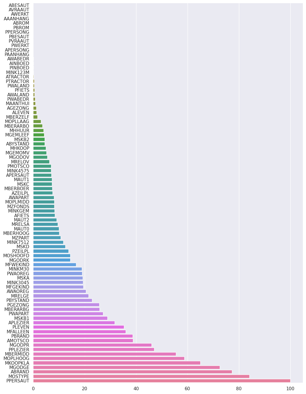
We can see that PPERSAUT is the most important feature in our data (this variable refers to the customer’s Contribution Car Policies, it quantifies the level of contribution a car customer makes towards insurance policies where \(0\) means he doesn’t contribute much to car policies and \(1\) to \(8\) are varying levels of contribution).

To read more about the data.

We can also see multiple features with high importance values.

(c)

y_prob = gbc_results.predict_proba(X_test)
y_pred = np.where(y_prob[:,1] > 0.2, 'Yes', 'No')

print(f"Accuracy: {accuracy_score(y_test, y_pred)}")
print(f"Precision: {precision_score(y_test, y_pred, pos_label='Yes'):.4f}")
print(f"Recall: {recall_score(y_test, y_pred, pos_label='Yes'):.4f}")

confusion_table(y_pred, y_test)

Accuracy: 0.9072998755703028
Precision: 0.1653
Recall: 0.1349

Truth	No	Yes
Predicted
No	4336	250
Yes	197	39

The fraction of people predicted to make a purchase that do in fact make one (the precision) is:

\[ Precision = 0.1653 \]

Now we’ll fit a KNN and a LogisticRegression model to compare them against the Boosting model.

First the KNN model. We’ll use cross-validation to choose the number of neighbors and try to maximize the precision score.

knn = KNN()
kfold = skm.KFold(5,
                  shuffle=True,
                  random_state=2)

custom_scorer = make_scorer(precision_score, pos_label='Yes', zero_division=0)

grid = skm.GridSearchCV(knn,
                        {'n_neighbors': np.arange(1, 20)},
                        cv=kfold,
                        scoring=custom_scorer).fit(X_train, y_train)
grid.best_params_

{'n_neighbors': 4}

y_pred = grid.best_estimator_.predict(X_test)

print(f"KNN Accuracy: {accuracy_score(y_test, y_pred):.4f}")
print(f"KNN Precision: {precision_score(y_test, y_pred, pos_label='Yes'):.4f}")
print(f"KNN Recall: {recall_score(y_test, y_pred, pos_label='Yes'):.4f}")

confusion_table(y_pred, y_test)

KNN Accuracy: 0.9376
KNN Precision: 0.2000
KNN Recall: 0.0138

Truth	No	Yes
Predicted
No	4517	285
Yes	16	4

Now for logistic regression.

lr = skl.LogisticRegression(fit_intercept=True, max_iter=1000)
lr_results = lr.fit(X_train, y_train)

y_prob = lr_results.predict_proba(X_test)
y_pred = np.where(y_prob[:,1] > 0.2, 'Yes', 'No')

print(f"LR Accuracy: {accuracy_score(y_test, y_pred):.4f}")
print(f"LR Precision: {precision_score(y_test, y_pred, pos_label='Yes'):.4f}")
print(f"LR Recall: {recall_score(y_test, y_pred, pos_label='Yes'):.4f}")

confusion_table(y_pred, y_test)

LR Accuracy: 0.9015
LR Precision: 0.1771
LR Recall: 0.1765

Truth	No	Yes
Predicted
No	4296	238
Yes	237	51

We can see that KNN and logistic regression do pretty well on this data set, and can achieve results comparable to or even better than boosting here, however the choice of the best model mostly depends on business needs, for this type of problem picking the model with the higher precision or recall depends on how expensive missing a potential buyer or targeting a non-buyer (assuming postive predictions get some form of specialized marketing or offers) is for the business.

Q12.

We’ll answer this question for the Credit dataset from the ISLP package, for info on the dataset click here.

credit = load_data('Credit')
credit.head()

	ID	Income	Limit	Rating	Cards	Age	Education	Gender	Student	Married	Ethnicity	Balance
0	1	14.891	3606	283	2	34	11	Male	No	Yes	Caucasian	333
1	2	106.025	6645	483	3	82	15	Female	Yes	Yes	Asian	903
2	3	104.593	7075	514	4	71	11	Male	No	No	Asian	580
3	4	148.924	9504	681	3	36	11	Female	No	No	Asian	964
4	5	55.882	4897	357	2	68	16	Male	No	Yes	Caucasian	331

credit.info()

<class 'pandas.core.frame.DataFrame'>
RangeIndex: 400 entries, 0 to 399
Data columns (total 12 columns):
 #   Column     Non-Null Count  Dtype   
---  ------     --------------  -----   
 0   ID         400 non-null    int64   
 1   Income     400 non-null    float64 
 2   Limit      400 non-null    int64   
 3   Rating     400 non-null    int64   
 4   Cards      400 non-null    int64   
 5   Age        400 non-null    int64   
 6   Education  400 non-null    int64   
 7   Gender     400 non-null    category
 8   Student    400 non-null    category
 9   Married    400 non-null    category
 10  Ethnicity  400 non-null    category
 11  Balance    400 non-null    int64   
dtypes: category(4), float64(1), int64(7)
memory usage: 27.2 KB

credit.describe()

	ID	Income	Limit	Rating	Cards	Age	Education	Balance
count	400.000000	400.000000	400.000000	400.000000	400.000000	400.000000	400.000000	400.000000
mean	200.500000	45.218885	4735.600000	354.940000	2.957500	55.667500	13.450000	520.015000
std	115.614301	35.244273	2308.198848	154.724143	1.371275	17.249807	3.125207	459.758877
min	1.000000	10.354000	855.000000	93.000000	1.000000	23.000000	5.000000	0.000000
25%	100.750000	21.007250	3088.000000	247.250000	2.000000	41.750000	11.000000	68.750000
50%	200.500000	33.115500	4622.500000	344.000000	3.000000	56.000000	14.000000	459.500000
75%	300.250000	57.470750	5872.750000	437.250000	4.000000	70.000000	16.000000	863.000000
max	400.000000	186.634000	13913.000000	982.000000	9.000000	98.000000	20.000000	1999.000000

credit.describe(include='category')

	Gender	Student	Married	Ethnicity
count	400	400	400	400
unique	2	2	2	3
top	Female	No	Yes	Caucasian
freq	207	360	245	199

We’ll use Balance as our response variable which represents average credit card balance in USD.

model = MS(credit.columns.drop('Balance'), intercept=False)
D = model.fit_transform(credit)
feature_names = list(D.columns)
X = np.asarray(D)
y = credit['Balance']

X_train, X_test, y_train, y_test = skm.train_test_split(X, y, test_size=0.3, random_state=1)

Boosting:

credit_boost = GBR(n_estimators=1000,
                    random_state=1).fit(X_train, y_train)
boost_MSE = np.mean((y_test - credit_boost.predict(X_test))**2)
boost_MSE

8938.816355567129

Bagging:

credit_bagging = RF(n_estimators=1000, 
                    max_features=X_train.shape[1],
                    random_state=1).fit(X_train, y_train)
bagging_MSE = np.mean((y_test - credit_bagging.predict(X_test))**2)
bagging_MSE

14346.337228441666

Random Forests (\(m = \sqrt{p}\)):

credit_rf = RF(n_estimators=1000, 
               max_features='sqrt',
               random_state=1).fit(X_train, y_train)
rf_MSE = np.mean((y_test - credit_rf.predict(X_test))**2)
rf_MSE

28888.775582383332

BART:

credit_bart = BART(random_state=1, burnin=300, ndraw=1000).fit(X_train, y_train)
bart_MSE = np.mean((y_test - credit_bart.predict(X_test))**2)
bart_MSE

13270.316940363333

Linear Regression:

lr = skl.LinearRegression().fit(X_train, y_train)
lr_MSE = np.mean((y_test - lr.predict(X_test))**2)
lr_MSE

11660.013638016124

print(f"Boosting RMSE         : {np.sqrt(boost_MSE):.4f}")
print(f"Bagging RMSE          : {np.sqrt(bagging_MSE):.4f}")
print(f"Random Forests RMSE   : {np.sqrt(rf_MSE):.4f}")
print(f"BART RMSE             : {np.sqrt(bart_MSE):.4f}")
print(f"Linear Regression RMSE: {np.sqrt(lr_MSE):.4f}")

Boosting RMSE         : 94.5453
Bagging RMSE          : 119.7762
Random Forests RMSE   : 169.9670
BART RMSE             : 115.1969
Linear Regression RMSE: 107.9815

credit['Balance'].mean(), credit['Balance'].std()

(520.015, 459.75887738938314)

We can see that boosting does the best on this dataset with no parameter fine-tuning, surprisingly though linear regression comes in 2nd place with an RMSE of \(107\), while the other tree methods lag pretty far behind, which indicates that there might be strong linearities in the underlying relationships.