Ch11: Survival Analysis and Censored Data

import matplotlib.pyplot as plt
import numpy as np
import pandas as pd
import seaborn as sns

sns.set_theme()

%matplotlib inline

from ISLP import load_data
from ISLP.models import ModelSpec as MS
from lifelines import CoxPHFitter, KaplanMeierFitter
from lifelines.statistics import logrank_test

Conceptual

Q1

(a) Independent, as censoring the patients whose phone numbers start with “2” doesn’t give us any information about the time to disease relapse for the patient.

(b) Not independent, as censoring patients whose ages exceed \(99\) years old is directly related to the event being measured (longevity).

(c) Not independent, as patients who are very sick are likely to have shorter lives, and the variable of interest here is longevity.

(d) Not independent, because censoring here is caused directly by the event (finding work).

(e) Not independent, because censoring is again caused directly by the event happening early (giving birth).

(f) Not independent, because censoring is directly related to the variable studied (years of education), a lot of residents who have higher years of education will likely be censored.

(g) Independent, because the duration of the study is pre-determined to be \(5\) years which is unrelated to the prognosis of any of the patients.

(h) Independent, since the components have no difference in quality, the censoring time doesn’t tell us which is likely to last longer.

(i) Not independent, as knowing the censoring time tells which of the components will last longer since we know components from the older factory are of higher quality.

Q2

(a)

1. Not censored.

2. Censored.

3. Censored.

4. Not censored.

(b)

1. \(c_1\) is not known.

2. \(c_2 = 2 \space \text{years}\)

3. \(c_3 = 1.5 \space \text{years}\)

4. \(c_4\) is not known.

(c)

1. \(t_1 = 1.2 \space \text{years}\)

2. \(t_2\) is not known.

3. \(t_3\) is not known.

4. \(t_4 = 0.2 \space \text{years}\)

(d)

1. \(y_1 = 1.2 \space \text{years}\)

2. \(y_2 = 2 \space \text{years}\)

3. \(y_3 = 1.5 \space \text{years}\)

4. \(y_4 = 0.2 \space \text{years}\)

(e)

1. \(\delta_1 = 1\)

2. \(\delta_2 = 0\)

3. \(\delta_3 = 0\)

4. \(\delta_4 = 1\)

Q3

We have 2 non-censored events (phone replacements) so:

\[ K = 2 \]

\( d_k \): The unique event times for non-censored participants.

\[ d_1 = 0.2 \text{ years} \quad d_2 = 1.2 \text{ years} \]

\( r_k \): The number of phones available for replacement just before \(d_k\).

\[ r_1 = 4 \quad r_2 = 3 \]

\( q_k \): The number of phones replaced at time \(d_k\).

\[ q_1 = 1 \quad q_2 = 1 \]

Q4

(a) The estimated probability past a time \(d_k\) is:

\[ \hat S(d_k) = \prod_{j=1}^k \left( \frac{r_j - q_j}{r_j} \right) \]

For a time \(t\) that’s greater than \(d_k\) and less than \(d_{k+1}\):

\[ \hat S(t) = \hat S(d_k) \]

For \(t = 50\):

\[ \hat S(50) = \hat S(d_2) = \hat S(37.2) \]

Which means the estimated probability of survival past \(50\) days is the same as that for \(37.2\) days, which is:

\[ \hat S(d_2) = \left( \frac{r_2 - q_2}{r_2} \right) \times \left( \frac{r_1 - q_1}{r_1} \right) \]

We can easily find the values for \(r_j\) and \(q_j\) from the table.

\[ r_1 = 5 \quad q_1 = 1 \]

\[ r_2 = 4 \quad q_2 = 1 \]

Plugging in the equation above:

r1 = 5
q1 = 1
r2 = 4
q2 = 1
S = (r2 - q2) / r2 * (r1 - q1) / r1
S

0.6

\[ \hat S(50) = 60\% \]

(b)

\[\begin{split} \hat S(t) = \begin{cases} 1 & \text{if} \space t \lt 26.5 \\ 0.8 & \text{if} \space 26.5 \le t \lt 37.2 \\ 0.6 & \text{if} \space 36.2 \le t \lt 57.3 \\ 0.4 & \text{if} \space t \ge 57.3 \\ \end{cases} \end{split}\]

Q5

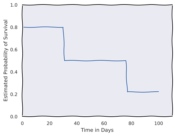
with plt.xkcd():
    plt.rcParams["font.family"] = "DejaVu Sans"  # to get rid of xkcd font warnings

    def S(t):
        if t < 31:
            return 0.8
        elif 31 <= t < 77:
            return 0.5
        elif t >= 77:
            return 0.22

    t = np.linspace(0, 100, 101)
    s = np.vectorize(S, otypes=[float])(t)

    plt.plot(t, s)
    plt.xlabel("Time in Days")
    plt.ylabel("Estimated Probability of Survival")
    plt.xlim([0, 110])
    plt.ylim([0, 1])

Q6

(a)

\(\delta_i\): The censoring indicator variable.

\[ \delta_1 = 1 \quad \delta_2 = 0 \quad \delta_3 = 1 \quad \delta_4 = 0 \]

We have 2 non-censored events so:

\[ K = 2 \]

\( d_k \): The unique event times for non-censored patients.

\[ d_1 = 150 \space \text{days} \quad d_2 = 300 \space \text{days} \]

\( r_k \): The number of patients at risk just before \(d_k\).

\[ r_1 = 4 \quad r_2 = 2 \]

\( q_k \): The number of deaths at time \(d_k\).

\[ q_1 = 1 \quad q_2 = 1 \]

(b)

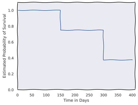
with plt.xkcd():
    plt.rcParams["font.family"] = "DejaVu Sans"  # to get rid of xkcd font warnings

    def S(t):
        if t < 150:
            return 1
        elif 150 <= t < 300:
            return (4 - 1) / 4
        elif t >= 300:
            return ((2 - 1) / 2) * ((4 - 1) / 4)

    t = np.arange(0, 401)
    s = np.vectorize(S, otypes=[float])(t)

    plt.plot(t, s)
    plt.xlabel("Time in Days")
    plt.ylabel("Estimated Probability of Survival")
    plt.xlim([0, 410])
    plt.ylim([0, 1.1])

(c) The probability that the event happens within \(200\) days is:

\[ 1 - \hat S(200) = 1 - 0.75 = 0.25 = 25\% \]

The probability that the event doesn’t occur within \(310\) days is:

\[ \hat S(310) = 0.375 = 37.5\% \]

(d)

This would be the expression for that estimated survival curve:

\[\begin{split} \hat S(t) = \begin{cases} 1 & \text{if} \space t < 150 \\ 0.75 & \text{if} \space 150 \le t < 300 \\ 0.375 & \text{if} \space t \ge 300 \\ \end{cases} \end{split}\]

Q7

(a) From the definition of the hypergeometric distribution (wikipedia’s):

The probability of \(k\) successes (random draws for which the object drawn has a specified feature) in \(n\) draws, without replacement, from a finite population of size \(N\) that contains exactly \(K\) objects with that feature, wherein each draw is either a success or a failure.

\[ P(X=k) = \frac{\binom{K}{k} \binom{N-K}{n-k}}{\binom{N}{n}} \]

For our case that would be the probability of \(q_{1k}\) failures, in \(r_{1k}\) draws, without replacement, from a risk set of \(r_k\) observations that contains a total of \(q_k\) failures.

\[ P(X=q_{1k}) = \frac{\binom{q_k}{q_{1k}} \binom{r_k-q_k}{r_{1k}-q_{1k}}}{\binom{r_k}{r_{1k}}} \]

The equivalent variable for each

\[ k = q_{1k} \quad K = q_k \quad n = r_{1k} \quad N = r_k \]

(b) Given the mean and variance of the hypergeometric distribution:

\[ E[X] = n \frac{K}{N} = r_{1k} \frac{q_k}{r_k} = \mu_k \]

\[ Var(X) = n \frac{K}{N} \frac{N-K}{N} \frac{N-n}{N-1} = r_{1k} \frac{q_k}{r_k} \frac{r_k-q_k}{r_k} \frac{r_k-r_{1k}}{r_k-1} = Var(q_{1k}) \]

Comparing to the equations in the book (11.5) and (11.6) we can see that they’re equivalent.

Q8

The given function definitions:

\[ S(t) = \Pr(T > t) \]

\[ h(t) = \lim_{\Delta t \to 0} \frac{\Pr(t < T \leq t + \Delta t | T > t)}{\Delta t} \]

\[ f(t) = \lim_{\Delta t \to 0} \frac{\Pr(t < T \leq t + \Delta t)}{\Delta t} \]

Defining \(F(t) = 1 - S(t)\):

\[ F(t) = 1 - \Pr(T \gt t) = \Pr(T \lt t) \]

---

Proving that \(f(t) = dF(t)/dt\) holds:

\[ \frac{d}{dt} F(t) = \frac{d}{dt} \Pr(T < t) \]

Using the definition of the derivative to expand the R.H.S:

\[ \frac{d}{dx} f(x) = \lim_{\Delta x \to 0} \frac{f(x + \Delta x) - f(x)}{\Delta x} \]

\[ \frac{d}{dt} \Pr(T < t) = \lim_{\Delta t \to 0} \frac{\Pr(T < t + \Delta t) - \Pr(T < t)}{\Delta t} \]

Simplifying the expression on the right:

\[ \frac{d}{dt} \Pr(T < t) = \lim_{\Delta t \to 0} \frac{\Pr(t < T \leq t + \Delta t)}{\Delta t} = f(t) \]

Thus, we have shown that \(f(t) = dF(t)/dt\).

---

Prove that:

\[\begin{split} S(t) = \exp\left(-\int_{0}^{t} h(u)du \right) \\ \end{split}\]

From the book (11.10):

\[ h(t) = \frac{f(t)}{S(t)} \]

Using the equation we proved eariler:

\[ h(t) = \frac{1}{S(t)} \frac{dF(t)}{dt} \]

Substituting for \(h(u)\) then doing a change of variables using \(F(u) = 1 - S(u)\) and \(dF(u) = -dS(u)\):

\[\begin{align*} S(t) &= \exp\left(-\int_{0}^{t} h(u)du \right) \\ &= \exp \left( -\int_{0}^{t} \frac{1}{S(u)} \frac{dF(u)}{du} du \right) \\ &= \exp \left( -\int_{S(0)}^{S(t)} \frac{1}{S(u)} -dS(u) \right) \\ &= \exp \left( \ln(S(u))\biggr\rvert^{S(t)}_{S(0)} \right) \\ &= \exp \left( \ln(S(t)) - \ln(S(0) )\right) \end{align*} \]

Knowing that the probability of survival at time \(0\) is \(1\):

\[ S(0) = 1 \]

Substituting above:

\[\begin{align*} &= \exp(\ln(S(t)) - \ln(1)) \\ &= \exp(\ln(S(t))) \\ &= S(t) \end{align*}\]

Which is what we set out to prove.

Q9

(a) Given that:

\[\begin{align*} f(t) = \lambda \exp(-\lambda t) \\ F(t) = 1 - S(t) \\ f(t) = dF(t)/dt \\ \end{align*}\]

Show that:

\[ S(t) = \exp(-\lambda t) \]

Taking the antiderivative of \(f(t)\) to find \(F(t)\):

\[ F(t) = \int_{0}^{t} f(\tau) d\tau \]

Substituting for \(F(t)\) and \(f(t)\):

\[\begin{align*} S(t) &= 1 - \int_{0}^{t} \lambda \exp(-\lambda \tau) d\tau \\ &= 1 - (-\exp(- \lambda t) \biggr \rvert_{0}^{t}) \\ &= 1 - (-\exp(-\lambda t) + \exp(0)) \\ &= 1 - (1 - \exp(-\lambda t)) \\ &= \exp(-\lambda t) \\ \end{align*}\]

which is what we set out to prove.

(b)

The likelihood of the \(i\text{th}\) observation is:

\[\begin{align*} L_i &= \begin{cases} f(y_i) \quad \text{ if the ith observation is not censored}\\ S(y_i) \quad \text{ if the ith observation is censored} \\ \end{cases} \\ &= f(y_i)^{\delta_i} S(y_i)^{1 - \delta_i} \\ &= (\lambda \exp(-\lambda y_i))^{\delta_i} (\exp(-\lambda y_i))^{1 - \delta_i} \\ &= \lambda^{\delta_i} (\exp(-\lambda y_i))^{\delta_i} \frac{(\exp(-\lambda y_i))^{1}}{(\exp(-\lambda y_i))^{\delta_i}} \\ &= \lambda^{\delta_i} \exp(-\lambda y_i) \\ \end{align*}\]

The likelihood of the data is the product of the likelihoods for each of the \(n\) independent observations:

\[\begin{align*} L = \prod_{i = 1}^{n} L_i &= \prod_{i = 1}^{n} \lambda^{\delta_i} \exp(-\lambda y_i) \\ \end{align*}\]

(c)

To derive the maximum likelihood estimator for \(\lambda\), we start by maximizing the log of the likelihood we derived earlier:

\[\begin{align*} \ell(\lambda) = \ln(L) &= \ln \left( \prod_{i = 1}^{n} \lambda^{\delta_i} \exp(-\lambda y_i) \right) \\ &= \ln \left( \frac{\prod_{i = 1}^{n} \lambda^{\delta_i}}{\prod_{i = 1}^{n} \exp(\lambda y_i)} \right) \\ &= \ln \left( \lambda^{\sum_{i = 1}^n \delta_i} \right) - \left(\lambda \sum_{i = 1}^n y_i \right) \\ &= \left( \ln( \lambda) \sum_{i = 1}^n \delta_i \right) - \left(\lambda \sum_{i = 1}^n y_i \right) \\ \end{align*}\]

To maximize \(\ell(\lambda)\) we set its derivative equal to zero:

\[ \frac{d\ell(\lambda)}{d\lambda} = 0 \]

\[ \frac{d\ell(\lambda)}{d\lambda} = \frac{1}{\lambda} \sum_{i = 1}^n \delta_i - \sum_{i = 1}^n y_i \]

Equating it to \(0\) and solving for \(\lambda\):

\[\begin{split} \frac{1}{\lambda} \sum_{i = 1}^n \delta_i - \sum_{i = 1}^n y_i = 0 \\ \end{split}\]

The maximum likelihood estimate for \(\lambda\) would be:

\[\begin{split} \hat \lambda = \sum_{i = 1}^n \delta_i/\sum_{i = 1}^n y_i \\ \end{split}\]

Which is what we set out to prove.

(d) Since the mean of an \(Exp(\lambda)\) random variable is \(1/\lambda\), we can use the \(\text{MLE}\) for \(\lambda\) we got in part (c):

\[\begin{align*} \hat \mu &= \frac{1}{\hat \lambda} \\ &= \frac{1}{\sum_{i = 1}^n \delta_i/\sum_{i = 1}^n y_i} \\ &= \sum_{i = 1}^n y_i /\sum_{i = 1}^n \delta_i \\ \end{align*}\]

Applied

Q10

BrainCancer = load_data("BrainCancer")
BrainCancer.head()

	sex	diagnosis	loc	ki	gtv	stereo	status	time
0	Female	Meningioma	Infratentorial	90	6.11	SRS	0	57.64
1	Male	HG glioma	Supratentorial	90	19.35	SRT	1	8.98
2	Female	Meningioma	Infratentorial	70	7.95	SRS	0	26.46
3	Female	LG glioma	Supratentorial	80	7.61	SRT	1	47.80
4	Male	HG glioma	Supratentorial	90	5.06	SRT	1	6.30

BrainCancer.describe()

	ki	gtv	status	time
count	88.000000	88.000000	88.000000	88.000000
mean	81.022727	8.660795	0.397727	27.457500
std	10.508866	8.657576	0.492233	20.124412
min	40.000000	0.010000	0.000000	0.070000
25%	80.000000	2.500000	0.000000	10.392500
50%	80.000000	6.510000	0.000000	24.030000
75%	90.000000	12.100000	1.000000	41.597500
max	100.000000	34.640000	1.000000	82.560000

BrainCancer.describe(include="category")

	sex	diagnosis	loc	stereo
count	88	87	88	88
unique	2	4	2	2
top	Female	Meningioma	Supratentorial	SRT
freq	45	42	69	65

BrainCancer.info()

<class 'pandas.core.frame.DataFrame'>
RangeIndex: 88 entries, 0 to 87
Data columns (total 8 columns):
 #   Column     Non-Null Count  Dtype   
---  ------     --------------  -----   
 0   sex        88 non-null     category
 1   diagnosis  87 non-null     category
 2   loc        88 non-null     category
 3   ki         88 non-null     int64   
 4   gtv        88 non-null     float64 
 5   stereo     88 non-null     category
 6   status     88 non-null     int64   
 7   time       88 non-null     float64 
dtypes: category(4), float64(2), int64(2)
memory usage: 3.8 KB

(a)

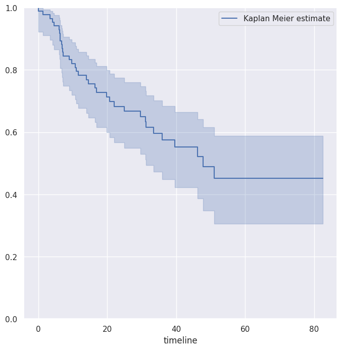
fig, ax = plt.subplots(figsize=(8, 8))
ax.set_ylim([0,1])
km = KaplanMeierFitter()
km_brain = km.fit(BrainCancer["time"], BrainCancer["status"])
km_brain.plot(label="Kaplan Meier estimate", ax=ax);

(b) We’ll use a modified version of the boot_SE function we used in chapter 5:

def boot_SE(
    func,
    df: pd.DataFrame,
    timepoints: np.ndarray = np.linspace(0, 100, 500),
    n=None,
    B=1000,
    seed=0,
):
    """
    Calculates the bootstrap standard error for a function that returns
    a lifelines fitter object.

    Args:
        func: A function that takes a DataFrame and indices and returns
              a fitted lifelines fitter object.
        df: The original DataFrame.
        timpoints: an array of timepoints which we calculate the SE at.
        n: The sample size for bootstrapping (defaults to D.shape[0]).
        B: The number of bootstrap samples.
        seed: Random seed for reproducibility.

    Returns:
        A pandas Series containing the standard error for the survival
        probability at each timepoint in the timepoints array.
    """
    rng = np.random.default_rng(seed)
    n = n or df.shape[0]
    fitters = []

    for _ in range(B):
        idx = rng.choice(df.index, n, replace=True)
        fitter = func(df, idx)
        fitters.append(fitter)

    predictions_list = []

    # Predict survival for each fitter at timepoints
    for i, fitter in enumerate(fitters):
        preds = fitter.predict(timepoints).rename(f"prediction_{i}")
        predictions_list.append(preds)

    predictions = pd.concat(predictions_list, axis=1)

    # calculate standard error 
    # (both methods below are equivalent and calculate the population standard deviation)
    
    # first_ = predictions.sum(axis=1)
    # second_ = (predictions**2).sum(axis=1)
    # se = np.sqrt(second_ / B - (first_ / B) ** 2)
    
    se = predictions.std(axis=1, ddof=0)

    return se

Defining a boot_fn function that fits the Kaplan-Meier survival curve:

def boot_fn(df: pd.DataFrame, idx: np.ndarray):
    data = df.loc[idx]

    km = KaplanMeierFitter()
    km_brain = km.fit(data["time"], data["status"])
    return km_brain

timepoints = np.linspace(0, 85, 500)

boot_std_error = boot_SE(
    boot_fn, df=BrainCancer, timepoints=timepoints, n=88, B=200, seed=42
)

km_brain = KaplanMeierFitter().fit(BrainCancer["time"], BrainCancer["status"])
surv_curve = km_brain.survival_function_at_times(timepoints)
pos_std = surv_curve + boot_std_error
neg_std = surv_curve - boot_std_error

fig, ax = plt.subplots(figsize=(8, 8))
ax.plot(surv_curve, label="Kaplan Meier estimate")
ax.plot(pos_std, color="gray", linestyle="--", label="Bootstrap SE upper bound")
ax.plot(neg_std, color="gray", linestyle="--", label="Bootstrap SE lower bound")
ax.fill_between(surv_curve.index, neg_std, pos_std, color="gray", alpha=0.2)
ax.set_ylim([0,1])
ax.set_xlabel("timeline")
ax.legend()
plt.show()

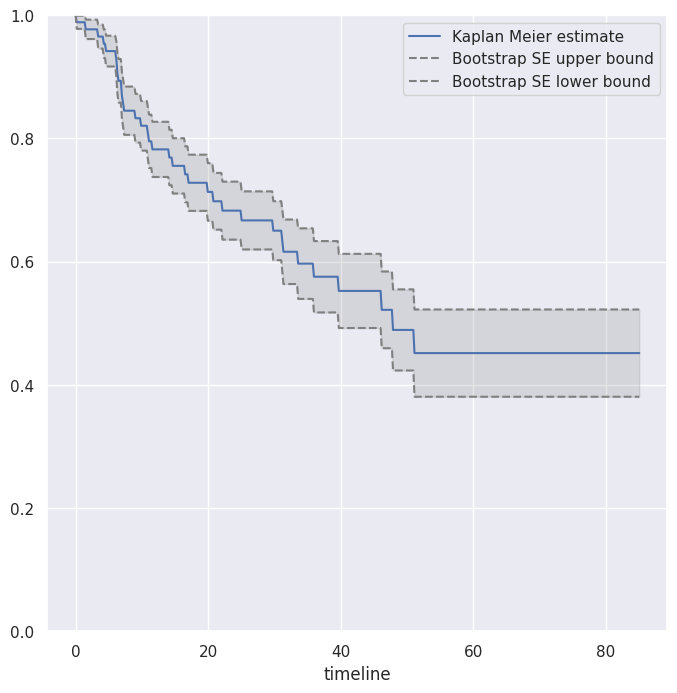
We can see that the bootstrap SE estimate band is quite a bit narrower than the one from the Kaplan-Meier fitter.

(c)

cleaned = BrainCancer.dropna()
all_MS = MS(cleaned.columns, intercept=False)
all_df = all_MS.fit_transform(cleaned)
fit_all = CoxPHFitter().fit(all_df,
                      'time',
                      'status')
fit_all.summary[['coef', 'se(coef)', 'p']]

	coef	se(coef)	p
covariate
sex[Male]	0.183748	0.360358	0.610119
diagnosis[LG glioma]	-1.239530	0.579555	0.032455
diagnosis[Meningioma]	-2.154566	0.450524	0.000002
diagnosis[Other]	-1.268870	0.617672	0.039949
loc[Supratentorial]	0.441195	0.703669	0.530665
ki	-0.054955	0.018314	0.002693
gtv	0.034293	0.022333	0.124661
stereo[SRT]	0.177778	0.601578	0.767597

We can see statistically significant p-values for the coefficients of ki, LG glioma, Meningioma, other.

(d) First we’ll group the single ki == 40 with the ki == 60 observations.

cleaned.loc[cleaned['ki'] == 40, 'ki'] = 60

Now we’ll adjust for other predictors, using the mode for categorical variables and the mean for numerical ones.

levels = sorted(cleaned['ki'].unique(), reverse=True)
def representative(series):
    if hasattr(series.dtype, 'categories'):
        return pd.Series.mode(series)
    else:
        return series.mean()
modal_data = cleaned.apply(representative, axis=0)

modal_df = pd.DataFrame(
              [modal_data.iloc[0] for _ in range(len(levels))])
modal_df['ki'] = levels
modal_df

	sex	diagnosis	loc	ki	gtv	stereo	status	time
0	Female	Meningioma	Supratentorial	100	8.687011	SRT	0.402299	27.188621
0	Female	Meningioma	Supratentorial	90	8.687011	SRT	0.402299	27.188621
0	Female	Meningioma	Supratentorial	80	8.687011	SRT	0.402299	27.188621
0	Female	Meningioma	Supratentorial	70	8.687011	SRT	0.402299	27.188621
0	Female	Meningioma	Supratentorial	60	8.687011	SRT	0.402299	27.188621

modal_X = all_MS.transform(modal_df)
modal_X.index = levels
modal_X

	sex[Male]	diagnosis[LG glioma]	diagnosis[Meningioma]	diagnosis[Other]	loc[Supratentorial]	ki	gtv	stereo[SRT]	status	time
100	0.0	0.0	1.0	0.0	1.0	100	8.687011	1.0	0.402299	27.188621
90	0.0	0.0	1.0	0.0	1.0	90	8.687011	1.0	0.402299	27.188621
80	0.0	0.0	1.0	0.0	1.0	80	8.687011	1.0	0.402299	27.188621
70	0.0	0.0	1.0	0.0	1.0	70	8.687011	1.0	0.402299	27.188621
60	0.0	0.0	1.0	0.0	1.0	60	8.687011	1.0	0.402299	27.188621

predicted_survival = fit_all.predict_survival_function(modal_X)
predicted_survival

	100	90	80	70	60
0.07	0.999280	0.998753	0.997840	0.996261	0.993532
1.18	0.999280	0.998753	0.997840	0.996261	0.993532
1.41	0.998484	0.997374	0.995455	0.992140	0.986421
1.54	0.998484	0.997374	0.995455	0.992140	0.986421
2.03	0.998484	0.997374	0.995455	0.992140	0.986421
...	...	...	...	...	...
65.02	0.877517	0.797428	0.675589	0.506907	0.308173
67.38	0.877517	0.797428	0.675589	0.506907	0.308173
73.74	0.877517	0.797428	0.675589	0.506907	0.308173
78.75	0.877517	0.797428	0.675589	0.506907	0.308173
82.56	0.877517	0.797428	0.675589	0.506907	0.308173

85 rows × 5 columns

fig, ax = plt.subplots(figsize=(8, 8))
predicted_survival.plot(ax=ax);

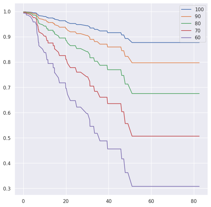
We can see that the plot matches what we understand from the coefficients of the fitted model, that a higher ki value is associated with lower risk, i.e. longer survival times.

Q11

Observation (Y)	Censoring Indicator (\(\delta\))	Covariate (X)
26.5	1	0.1
37.2	1	11
57.3	1	-0.3
90.8	0	2.8
20.2	0	1.8
89.8	0	0.4

TABLE 11.4.

data = {
    'y': [26.5, 37.2, 57.3, 90.8, 20.2, 89.8],
    'delta': [1, 1, 1, 0, 0, 0],
    'x': [0.1, 11, -0.3, 2.8, 1.8, 0.4]
}
df = pd.DataFrame(data)
df

	y	delta	x
0	26.5	1	0.1
1	37.2	1	11.0
2	57.3	1	-0.3
3	90.8	0	2.8
4	20.2	0	1.8
5	89.8	0	0.4

(a) Splitting the data into two groups:

df.loc[df['x'] < 2, 'group'] = "Group1"
df

	y	delta	x	group
0	26.5	1	0.1	Group1
1	37.2	1	11.0	NaN
2	57.3	1	-0.3	Group1
3	90.8	0	2.8	NaN
4	20.2	0	1.8	Group1
5	89.8	0	0.4	Group1

df.loc[df['x'] >= 2, 'group'] = "Group2"
df

	y	delta	x	group
0	26.5	1	0.1	Group1
1	37.2	1	11.0	Group2
2	57.3	1	-0.3	Group1
3	90.8	0	2.8	Group2
4	20.2	0	1.8	Group1
5	89.8	0	0.4	Group1

df['group'] = df['group'].astype('category')

fig, ax = plt.subplots(figsize=(8, 8))
for group_name, group in df.groupby('group', observed=True):
    km = KaplanMeierFitter().fit(group['y'], group['delta'])
    km.plot(label=f"{group_name}", ax=ax)

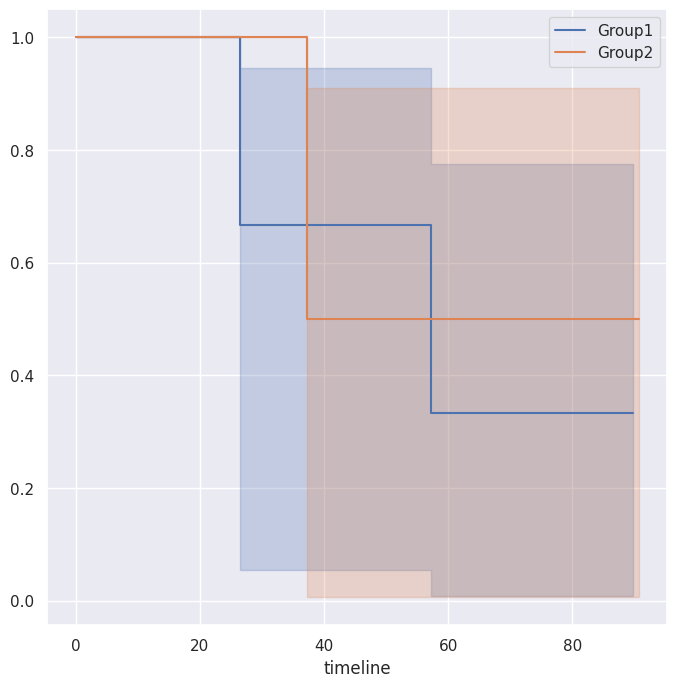
Looking at the fitted Kaplan-Meier curves, I can’t see a big difference between the two groups’ survival curves.

(b)

cols = ['y', 'delta', 'group']
design = MS(cols, intercept=False)
group_df = design.fit_transform(df)
group_df

	y	delta	group[Group2]
0	26.5	1	0.0
1	37.2	1	1.0
2	57.3	1	0.0
3	90.8	0	1.0
4	20.2	0	0.0
5	89.8	0	0.0

cox_fit = CoxPHFitter().fit(group_df,
                            'y',
                            'delta')
cox_fit.summary[['coef', 'se(coef)', 'p']]

	coef	se(coef)	p
covariate
group[Group2]	-0.340143	1.235876	0.783144

np.e**-0.340143

0.7116685468836035

The estimated coefficient is \(-0.340143\). Group1 is encoded as the baseline here, so we can interpret the coefficient to mean that the risk associated with Group2 \((e^{-0.340143} = 0.71167)\) is around \(30\%\) less than the risk associated with Group1. Since the p-value is \(0.783\) we have no evidence to believe that the coefficient’s true value is non-zero.

(c)

We can perform the log-rank test in to two ways either by calling log_likelihood_ratio_test() on the CoxPH model we fit earlier or using logrank_test() on the two groups. I’ll demonstrate both methods.

cox_fit.log_likelihood_ratio_test()

null_distribution	chi squared
degrees_freedom	1
test_name	log-likelihood ratio test

	test_statistic	p	-log2(p)
0	0.08	0.78	0.36

by_group = df.groupby('group', observed=True)
logrank_test(by_group.get_group('Group1')['y'],
             by_group.get_group('Group2')['y'],
             by_group.get_group('Group1')['delta'],
             by_group.get_group('Group2')['delta'])

t_0	-1
null_distribution	chi squared
degrees_of_freedom	1
test_name	logrank_test

	test_statistic	p	-log2(p)
0	0.08	0.78	0.35

The p-value from the log-rank test returned by both methods is exactly the same as the p-value returned by the Cox model fit in part (b), which is \(p = 0.78\).