Ch4: Classification

import numpy as np
import pandas as pd
import matplotlib.pyplot as plt
import seaborn as sns

import statsmodels.api as sm
from ISLP import load_data
from ISLP.models import (ModelSpec as MS,
                         summarize)

sns.set_theme()

%matplotlib inline

from ISLP import confusion_table
from sklearn.discriminant_analysis import \
     (LinearDiscriminantAnalysis as LDA,
      QuadraticDiscriminantAnalysis as QDA)
from sklearn.naive_bayes import GaussianNB
from sklearn.neighbors import KNeighborsClassifier
from sklearn.preprocessing import StandardScaler
from sklearn.model_selection import train_test_split
from sklearn.linear_model import LogisticRegression

Conceptual

Q1.

Starting with (4.2):

\[ p(X) = \frac{e^{\beta_0 + \beta_1 X}}{1 + e^{\beta_0 + \beta_1 X}} \]

Multiply both sides by:

\[ 1 + e^{\beta_0 + \beta_1 X} \ \]

To get:

\[ p(X) + p(X) e^{\beta_0 + \beta_1 X} = e^{\beta_0 + \beta_1 X} \]

Rearranging the terms:

\[ p(X) = e^{\beta_0 + \beta_1 X} - p(X) e^{\beta_0 + \beta_1 X} \]

Factoring out \(e^{\beta_0 + \beta_1 X}\) and dividing both sides by the remainder:

\[ \frac{p(X)}{1-p(X)} = e^{\beta_0 + \beta_1 X} \]

We get (4.3) which is what we set out to prove.

Q2.

\[ p_k(x) = \frac{\pi_k \frac{1}{\sqrt{2\pi}\sigma} \exp\left(-\frac{1}{2\sigma^2} (x - \mu_k)^2\right)} {\sum_{l=1}^{K} \pi_l \frac{1}{\sqrt{2\pi}\sigma} \exp\left(-\frac{1}{2\sigma^2} (x - \mu_l)^2\right)} \]

Taking the \( log \) of both sides:

\[ log(p_k(x)) = log(\pi_k \frac{1}{\sqrt{2\pi}\sigma} \exp\left(-\frac{1}{2\sigma^2} (x - \mu_k)^2\right)) - log(\sum_{l=1}^{K} \pi_l \frac{1}{\sqrt{2\pi}\sigma} \exp\left(-\frac{1}{2\sigma^2} (x - \mu_l)^2\right)) \]

\[ log(p_k(x)) = log(\pi_k) + log(\frac{1}{\sqrt{2\pi}\sigma}) + log(\exp\left(-\frac{1}{2\sigma^2} (x - \mu_k)^2\right))) - log(\sum_{l=1}^{K} \pi_l \frac{1}{\sqrt{2\pi}\sigma} \exp\left(-\frac{1}{2\sigma^2} (x - \mu_l)^2\right)) \]

To maximize the value of the function above over all k we only need to consider terms that vary with k:

\[ log(\pi_k) - \frac{1}{2\sigma^2} * (x^2 -2 \mu_k x + \mu_k^2) \]

\[ log(\pi_k) -\frac{1}{2\sigma^2} * x^2 +\frac{1}{\sigma^2} \mu_k x - \frac{1}{2\sigma^2} \mu_k^2 \]

The term \( -\frac{x^2}{2\sigma^2} \) is constant across all values of k so we can ignore it and the remaining 3 terms are what we have to consider:

\[ \delta_k(x) = x \cdot \frac{\mu_k}{\sigma^2} - \frac{\mu_k^2}{2\sigma^2} + \log(\pi_k) \]

Q3.

This question is similar to the previous question except for the assumption that \(\sigma_1^2 = ... = \sigma_K^2\) which we don’t apply here:

\[ p_k(x) = \frac{\pi_k \frac{1}{\sqrt{2\pi}\sigma_k} \exp\left(-\frac{1}{2\sigma_k^2} (x - \mu_k)^2\right)} {\sum_{l=1}^{K} \pi_l \frac{1}{\sqrt{2\pi}\sigma_l} \exp\left(-\frac{1}{2\sigma_l^2} (x - \mu_l)^2\right)} \]

Following the same steps used in the above question, taking the log and considering only terms that vary with k:

\[ log(p_k(x)) = log(\pi_k) + log(\frac{1}{\sqrt{2\pi}\sigma_k}) + log(\exp\left(-\frac{1}{2\sigma_k^2} (x - \mu_k)^2\right))) - log(\sum_{l=1}^{K} \pi_l \frac{1}{\sqrt{2\pi}\sigma_l} \exp\left(-\frac{1}{2\sigma_l^2} (x - \mu_l)^2\right)) \]

\[ log(\frac{\pi_k}{\sigma_k}) -\frac{1}{2\sigma_k^2} * x^2 +\frac{1}{\sigma_k^2} \mu_k x - \frac{1}{2\sigma_k^2} \mu_k^2 \]

We can see that the discriminant function takes the form:

\[ \delta_k(x) = log(\frac{\pi_k}{\sigma_k}) -\frac{x^2}{2\sigma_k^2} + x \frac{\mu_k}{\sigma_k^2} - \frac{\mu_k^2}{2\sigma_k^2} \]

Which is quadratic in x.

Q4.

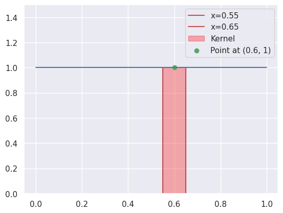
(a) To answer this question we can imagine a kernel of width 0.1 sweeping along the X-axis from 0 to 1, where the area of the kernel around a point X corresponds to the fraction of available observations we use to make a prediction for the response of test observation X.

The following figure just helps us visualise what we mean to do. And intuitivly the result should be close to 10% since it stays 10% for all points in the range [0.05, 0.95] and slightly decreases outside that range.

fig, ax = plt.subplots()
ax.set_ylim([0, 1.5])

# Plot the horizontal line
ax.plot([0, 1], [1, 1], c='b')  

# Add vertical red lines using ax.plot (absolute coordinates)
ax.plot([0.55, 0.55], [0, 1], c='r', label='x=0.55')  # Line from y=0 to y=1
ax.plot([0.65, 0.65], [0, 1], c='r', label='x=0.65')  # Line from y=0 to y=1

# Shade the area between the two vertical lines
ax.axvspan(0.55, 0.65, 0, 1/ax.get_ylim()[1], color='red', alpha=0.3, label='Kernel')

ax.scatter(0.6, 1, c='g', label='Point at (0.6, 1)')
ax.legend()

plt.show()

within = 0.1
lim = within/2
obs = np.linspace(0, 1, 1001)
used_obs = np.array([])
for i in obs:
    left = i - lim
    if left < 0:
        left = 0
    
    right = i + lim 
    if right > 1:
        right = 1
    # print(f'[{left:.2f}, {right:.2f}]')
    used_obs = np.append(used_obs, right - left)

plt.plot(obs, used_obs);
used_obs.mean()

0.09745254745254749

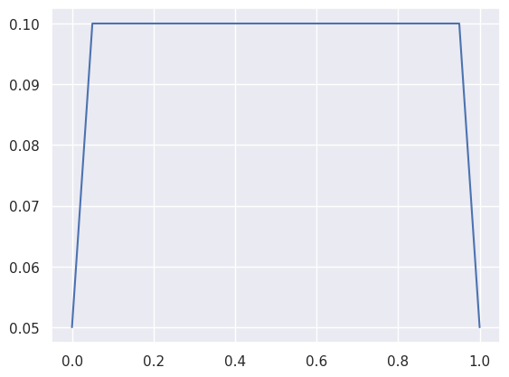
We can see that on average, the fraction of available observations we use to make the prediction is 9.75%.

(b) Extending the idea above from 2 dimensions (p = 1) to 3 dimensions (p = 2).

within = 0.10
lim = within/2
obs = np.arange(0, 1, 0.01)
p = 2
used_obs = []
for n in range(p):

    used_obs_dim = []
    for i in obs:
        minimum = i - lim
        if minimum < 0:
            minimum = 0
        
        max = i + lim 
        if max > 1:
            max = 1
            
        # print(f'[{min:.2f}, {max:.2f}]')
        used_obs_dim.append(max - minimum)
    used_obs.append(used_obs_dim)

used_obs = np.array(used_obs)

import operator 
from functools import reduce

grid = np.meshgrid(*used_obs, indexing="ij")

result = reduce(operator.mul, grid)
result.mean()

0.009506250000000008

We can see that on average we use 0.95% of the available observations to make the prediction.

(c)

Similar to what we did above we just extend the same ideas to a 101 dimensions (p = 100). Creating the grid for the data would be troublesome so we’ll just use the fact that from every dimension we use 9.75% of the data like so.

\[ 0.0975 ^ p \]

0.0975 ** 2

0.00950625

We can see that we get the same result we calculated above for p = 2.

0.0975 ** 100

7.951728986183188e-102

As we can see the value is so miniscule that we’re practically using almost 0% of the available observations to make a prediction.

(d) Looking at our answers from (a)-(c) we can see that the more predictors we use while considering a non-parametric method like KNN, the less test observations are used to make the prediction, since data points become very sparse in higher dimensions.

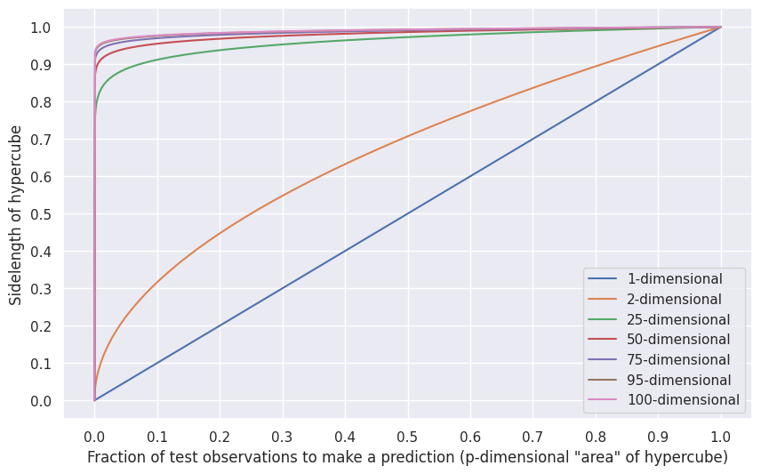
(e) To find the sidelength of the hypercube that contains 10% of the testing observations we just need to find the sidelength of a p-dimensional hypercube that has a p-dimensional “area” of 0.10.

\[ x ^ p = 0.10 \]

for \(p = 1\) that’d be:

\[ x = 0.10 \]

for \(p = 2\) that’d be:

np.power(0.10, 1/2)

0.31622776601683794

\[\begin{split} x = \sqrt{0.10} \\ x = 0.3163 \end{split}\]

for \( p = 100 \):

np.power(0.10, 1/100)

0.9772372209558108

\[\begin{split} x = \sqrt[^{100}]{0.10}\\ x = 0.977 \end{split}\]

We can see that for large values of p the sidelength of the hypercube gets so big to the point where it’s close to 1 but only 10% of test observations fall within the hypercube, which is a testament to how sparse data in high dimensional space gets.

I’ll create a plot to capture that relation for various values of p:

fig, ax = plt.subplots(figsize=(10, 6))
for p in [1, 2, 25, 50, 75, 95, 100]:
    x = np.linspace(0, 1, 1001)
    ax.plot(x, np.power(x, 1/p), label=f'{p}-dimensional')

ax.set_xticks(np.arange(0, 1.1, 0.1))
ax.set_yticks(np.arange(0, 1.1, 0.1))
ax.set_xlabel('Fraction of test observations to make a prediction (p-dimensional "area" of hypercube)')
ax.set_ylabel('Sidelength of hypercube')
ax.legend();

Q5.

(a) We expect QDA to perform better on the training set than LDA due to it being a more flexible model, however we expect LDA to perform better on the test set since it’d have less bias due to the Bayes decision boundary being linear.

(b) QDA would perform better on both the training and test sets, because here the increase in variance from using a more flexible model (QDA) is offset by a decrease in bias due to the Bayes decision boundary being non-linear.

(c) We expect it to improve, as the additional incurred cost in variance from choosing a more flexible classifer (QDA over LDA) is offset by the large sample size.

(d) False. Because the resulting increase in variance from using a more flexible model isn’t offset by any decrease in bias since the Bayes decision boundary is linear hence LDA would have a better test error rate than QDA.

Q6.

(a) We can simply do that using the formula:

\[ p(Hours, GPA) = \frac{e^{\beta_0 + \beta_1 * Hours + \beta_2 * GPA}}{1+e^{\beta_0 + \beta_1 * Hours + \beta_2 * GPA}} \]

b0 = -6 
b1 = 0.05
b2 = 1

def predict(Hours, GPA):
    numerator = np.exp(b0 + b1 * Hours + b2 * GPA)
    denominator = 1 + np.exp(b0 + b1 * Hours + b2 * GPA)
    
    return numerator / denominator

predict(40, 3.5)

0.37754066879814546

The student has a probability of 37.75% to get an A in that class.

(b) To find the amount of time he’s required to study to make his probability of getting an A 50% we just plug 50% for \(p\) and solve for \(Hours\):

\[ log(\frac{p}{1-p}) = \beta_0 + \beta_1 * Hours + \beta_2 * GPA \]

p = 0.5
GPA = 3.5
Hours = (np.log(p/(1-p)) - b0 - b2 * GPA)/b1
Hours

50.0

We see that he needs to study 10 more hours (for a total of 50 hours) to increase his probability of getting an A to 50%.

Q7.

From the given information we can see that the assumptions are the same as those for LDA, namely X follows a normal distribution with constant variance across the classes.

\[\begin{align*} \bar{X}_{Yes} = 10 \\ \bar{X}_{No} = 0 \\ \sigma_{Yes}^2 = \sigma_{No}^2 = 36 \\ \pi_{Yes} = 0.8 \\ \pi_{No} = 0.2 \end{align*}\]

Using Bayes’ theorem with the assumption that \(f_k(x)\) is normally distributed:

\[ p_k(x) = \frac{\pi_k \frac{1}{\sqrt{2\pi\sigma^2}} \exp\left(-\frac{1}{2\sigma^2} (x - \mu_k)^2\right)} {\sum_{l=1}^{K} \pi_l \frac{1}{\sqrt{2\pi\sigma^2}} \exp\left(-\frac{1}{2\sigma^2} (x - \mu_l)^2\right)} \]

def f(x, mean, variance, prior):
    return prior * (1/np.sqrt(2 * np.pi * variance)) * np.exp((-1/(2*variance)) * (x - mean)**2)

f(4, 10, 36, 0.8)/(f(4, 0, 36, 0.2) + f(4, 10, 36, 0.8))

0.7518524532975261

\[ p_{Yes}(4) = 0.7519 \]

We can see that a company that had a percentage profit of X = 4 last year has a probability of 75.19% to issue a dividend this year.

Q8.

We should still use logistic regression because it’s very likely that the KNN (with K=1) classifier overfit to the data resulting in a training error rate of around 0% and a test error rate of 36% which is higher than LR’s 30% test error rate.

Q9.

(a)

\[\begin{split} odds = \frac{p(X)}{1-p(X)} \\ \end{split}\]

\[ p(X) = \frac{odds}{1+ odds} \]

0.37/(1 + 0.37)

0.27007299270072993

27% of people with an odds of 0.37 of defaulting on their credit card will default.

(b)

0.16/(1 - 0.16)

0.1904761904761905

She has an odds of 0.19 that she’ll default.

Q10.

Starting with:

\[ log(\frac{Pr(Y = k | X = x)}{Pr(Y = K | X = x)}) = log(\frac{\pi_k f_k(x)}{\pi_K f_K(x)}) \]

And considering the case for \(p = 1\), where the means \(\mu_1, ..., \mu_K\) and variance \(\sigma^2\) are scalars:

\[ f_k(x) = \frac{1}{\sqrt{2 \pi \sigma^2}} exp(\frac{-(x-\mu_k)^2}{2\sigma^2}) \]

\[\begin{align*} log(\frac{\pi_k f_k(x)}{\pi_K f_K(x)}) &= log(\frac{\pi_k exp(\frac{-(x-\mu_k)^2}{2\sigma^2})}{\pi_K exp(\frac{-(x-\mu_K)^2}{2\sigma^2})}) \\ &= log(\pi_k exp(\frac{-(x-\mu_k)^2}{2\sigma^2})) - log(\pi_K exp(\frac{-(x-\mu_K)^2}{2\sigma^2})) \\ &= log(\pi_k) -\frac{(x-\mu_k)^2}{2\sigma^2} + \frac{(x-\mu_K)^2}{2\sigma^2} - log(\pi_K) \\ &= log(\frac{\pi_k}{\pi_K}) - \frac{1}{2\sigma^2} (x^2 - 2 \mu_k x + \mu_k^2) + \frac{1}{2\sigma^2} (x^2 - 2 \mu_K x + \mu_K^2) \\ &= log(\frac{\pi_k}{\pi_K}) - \frac{(\mu_K^2 - \mu_k^2)}{2\sigma^2} + \frac{(\mu_k - \mu_K)}{\sigma^2} x \\ &= a_k + b_k x \end{align*}\]

Where

\[ \begin{align}\begin{aligned}\begin{split} a_k = log(\frac{\pi_k}{\pi_K}) - \frac{(\mu_K^2 - \mu_k^2)}{2\sigma^2} \\ \end{split}\\b_k = \frac{(\mu_k - \mu_K)}{\sigma^2} \end{aligned}\end{align} \]

Q11.

Starting with:

\[ log(\frac{Pr(Y = k | X = x)}{Pr(Y = K | X = x)}) = log(\frac{\pi_k f_k(x)}{\pi_K f_K(x)}) \]

And considering the case for \(p > 1\), where the means \(\mu_1, ..., \mu_K\) are p-dimensional vectors, and \(\Sigma_1, ..., \Sigma_k\) are \(p \times p\) covariance matrices (A multivariate normal distribution):

\[\begin{align*} f_k(\mathbf{x}) &= \frac{1}{\sqrt{(2 \pi)^p det(\mathbf{\Sigma_k})}} exp(-\frac{1}{2}(\mathbf x- \mathbf{\mu_k})^T \mathbf{\Sigma_k}^{-1} (\mathbf x- \mathbf{\mu_k})) \\ &= (2 \pi)^{-p/2} det(\mathbf{\Sigma_k})^{-1/2} exp(-\frac{1}{2}(\mathbf x- \mathbf{\mu_k})^T \mathbf{\Sigma_k}^{-1} (\mathbf x- \mathbf{\mu_k})) \\ \end{align*}\]

\[\begin{align*} log(\frac{\pi_k f_k(\mathbf x)}{\pi_K f_K(\mathbf x)}) &= log(\frac{\pi_k det(\mathbf{\Sigma_k})^{-1/2} exp(-\frac{1}{2}(\mathbf x- \mathbf{\mu_k})^T \mathbf{\Sigma_k}^{-1} (\mathbf x- \mathbf{\mu_k}))}{\pi_K det(\mathbf{\Sigma_K})^{-1/2} exp(-\frac{1}{2}(\mathbf x- \mathbf{\mu_K})^T \mathbf{\Sigma_K}^{-1} (\mathbf x- \mathbf{\mu_K}))}) \\ &= log(\pi_k det(\mathbf{\Sigma_k})^{-1/2} ) -\frac{1}{2}(\mathbf x- \mathbf{\mu_k})^T \mathbf{\Sigma_k}^{-1} (\mathbf x- \mathbf{\mu_k}) - log(\pi_K det(\mathbf{\Sigma_K})^{-1/2} ) + \frac{1}{2}(\mathbf x- \mathbf{\mu_K})^T \mathbf{\Sigma_K}^{-1} (\mathbf x- \mathbf{\mu_K}) \\ &= log(\frac{\pi_k}{\pi_K}) + \frac{1}{2} log(\frac{det(\mathbf{\Sigma_K})}{det(\mathbf{\Sigma_k})} ) -\frac{1}{2}(\mathbf x- \mathbf{\mu_k})^T \mathbf{\Sigma_k}^{-1} (\mathbf x- \mathbf{\mu_k}) + \frac{1}{2}(\mathbf x- \mathbf{\mu_K})^T \mathbf{\Sigma_K}^{-1} (\mathbf x- \mathbf{\mu_K}) \\ &= log(\frac{\pi_k}{\pi_K}) + \frac{1}{2} log(\frac{det(\mathbf{\Sigma_K})}{det(\mathbf{\Sigma_k})} ) - \frac{1}{2} \mathbf x^T \mathbf{\Sigma_k}^{-1} \mathbf x + \mathbf{\mu_k}^T \mathbf{\Sigma_k}^{-1} x - \frac{1}{2} \mathbf{\mu_k}^T \mathbf{\Sigma_k}^{-1} \mu_k + \frac{1}{2}\mathbf x^T \mathbf{\Sigma_K}^{-1} \mathbf x - \mathbf{\mu_K}^T \mathbf{\Sigma_K}^{-1} x + \frac{1}{2} \mathbf{\mu_K}^T \mathbf{\Sigma_K}^{-1} \mu_K\\ &= log(\frac{\pi_k}{\pi_K}) + \frac{1}{2} log(\frac{det(\mathbf{\Sigma_K})}{det(\mathbf{\Sigma_k})} ) + \frac{1}{2} \mathbf x^T \mathbf(\mathbf{\Sigma_K}^{-1} - \mathbf{\Sigma_k}^{-1}) \mathbf x + (\mathbf{\mu_k}^T \mathbf{\Sigma_k}^{-1} - \mathbf{\mu_K}^T \mathbf{\Sigma_K}^{-1}) x + \frac{1}{2} (\mathbf{\mu_K}^T \mathbf{\Sigma_K}^{-1} \mu_K - \mathbf{\mu_k}^T \mathbf{\Sigma_k}^{-1} \mu_k)\\ &= log(\frac{\pi_k}{\pi_K}) + \frac{1}{2} log(\frac{det(\mathbf{\Sigma_K})}{det(\mathbf{\Sigma_k})} ) + \frac{1}{2} (\mathbf{\mu_K}^T \mathbf{\Sigma_K}^{-1} \mu_K - \mathbf{\mu_k}^T \mathbf{\Sigma_k}^{-1} \mu_k) + (\mathbf{\mu_k}^T \mathbf{\Sigma_k}^{-1} - \mathbf{\mu_K}^T \mathbf{\Sigma_K}^{-1}) x + \frac{1}{2} \mathbf x^T (\mathbf{\Sigma_K}^{-1} - \mathbf{\Sigma_k}^{-1}) \mathbf x \\ &= a_k + \sum^{p}_{j=1} b_{kj} x_j + \sum^{p}_{j=1} \sum^{p}_{l=1} c_{kjl} x_j x_l \end{align*}\]

Where

\[\begin{split} a_k = log(\frac{\pi_k}{\pi_K}) + \frac{1}{2} log(\frac{det(\mathbf{\Sigma_K})}{det(\mathbf{\Sigma_k})} ) + \frac{1}{2} (\mathbf{\mu_K}^T \mathbf{\Sigma_K}^{-1} \mu_K - \mathbf{\mu_k}^T \mathbf{\Sigma_k}^{-1} \mu_k) \\ \end{split}\]

And

\[ \begin{align}\begin{aligned}\begin{split} b_{kj} = (\mathbf{\mu_k}^T \mathbf{\Sigma_k}^{-1} - \mathbf{\mu_K}^T \mathbf{\Sigma_K}^{-1})_j\\ \end{split}\\c_{kjl} = \frac{1}{2} (\mathbf{\Sigma_K}^{-1} - \mathbf{\Sigma_k}^{-1})_{jl} \end{aligned}\end{align} \]

Note: The notation above is just a way of indexing, indicating that for example \(b_{kj}\) is the \(j\text{th}\) component of \((\mathbf{\mu_k}^T \mathbf{\Sigma_k}^{-1} - \mathbf{\mu_K}^T \mathbf{\Sigma_K}^{-1})\).

Q12.

(a)

\[\begin{align*} log(\frac{Pr(Y = orange | X = x)}{Pr(Y = apple | X = x)}) &= log(\frac{Pr(Y = orange | X = x)}{1 - Pr(Y = orange | X = x)}) \\ &= log(\frac{\frac{exp(\hat{\beta}_0 + \hat{\beta}_1 x)}{1 + exp(\hat{\beta}_0 + \hat{\beta}_1 x)}}{1 - \frac{exp(\hat{\beta}_0 + \hat{\beta}_1 x)}{1 + exp(\hat{\beta}_0 + \hat{\beta}_1 x)}}) \\ &= log(\frac{\frac{exp(\hat{\beta}_0 + \hat{\beta}_1 x)}{1 + exp(\hat{\beta}_0 + \hat{\beta}_1 x)}}{\frac{1}{1 + exp(\hat{\beta}_0 + \hat{\beta}_1 x)}}) \\ &= log(exp(\hat{\beta}_0 + \hat{\beta}_1 x)) \\ &= \hat{\beta}_0 + \hat{\beta}_1 x \end{align*}\]

The log odds of orange versus apple in my model is \(\hat{\beta}_0 + \hat{\beta}_1 x\)

(b)

\[\begin{align*} log(\frac{Pr(Y = orange | X = x)}{Pr(Y = apple | X = x)}) &= log(\frac{\frac{exp(\hat{\alpha}_{orange0} + \hat{\alpha}_{orange1} x)}{exp(\hat{\alpha}_{orange0} + \hat{\alpha}_{orange1} x) + exp(\hat{\alpha}_{apple0} + \hat{\alpha}_{apple1} x)}}{\frac{exp(\hat{\alpha}_{apple0} + \hat{\alpha}_{apple1} x)}{exp(\hat{\alpha}_{orange0} + \hat{\alpha}_{orange1} x) + exp(\hat{\alpha}_{apple0} + \hat{\alpha}_{apple1} x)}}) \\ &= log(\frac{exp(\hat{\alpha}_{orange0} + \hat{\alpha}_{orange1} x)}{exp(\hat{\alpha}_{apple0} + \hat{\alpha}_{apple1} x)}) \\ &= (\hat{\alpha}_{orange0} - \hat{\alpha}_{apple0}) + (\hat{\alpha}_{orange1} - \hat{\alpha}_{apple1}) x\\ \end{align*}\]

The log odds of orange versus apple in our friend’s model is \((\hat{\alpha}_{orange0} - \hat{\alpha}_{apple0}) + (\hat{\alpha}_{orange1} - \hat{\alpha}_{apple1}) x\)

(c) The given coefficients for our model:

\[\begin{align*} \hat{\beta}_0 &= 2 \\ \hat{\beta}_1 &= -1 \end{align*}\]

By equating the log odds results from both models:

\[\begin{split} \hat{\beta}_0 + \hat{\beta}_1 x = (\hat{\alpha}_{orange0} - \hat{\alpha}_{apple0}) + (\hat{\alpha}_{orange1} - \hat{\alpha}_{apple1}) x \\ \end{split}\]

\[\begin{split} \hat{\beta}_0 = (\hat{\alpha}_{orange0} - \hat{\alpha}_{apple0}) \\ \end{split}\]

\[ \hat{\beta}_1 = (\hat{\alpha}_{orange1} - \hat{\alpha}_{apple1}) \]

By equating the log odds results from both models:

\[\begin{split} \hat{\beta}_0 + \hat{\beta}_1 x = (\hat{\alpha}_{orange0} - \hat{\alpha}_{apple0}) + (\hat{\alpha}_{orange1} - \hat{\alpha}_{apple1}) x \\ \end{split}\]

\[\begin{split} \hat{\beta}_0 = (\hat{\alpha}_{orange0} - \hat{\alpha}_{apple0}) \\ \end{split}\]

\[ \hat{\beta}_1 = (\hat{\alpha}_{orange1} - \hat{\alpha}_{apple1}) \]

From this we can see that infinitely many solutions exist, basically any two values with a difference equal to the estimated \(\hat\beta\) coefficient would suffice.

\[\begin{split} \begin{aligned} \hat{\alpha}_{orange0} = 2 + c_0 \\ \hat{\alpha}_{apple0} = c_0 \\ \hat{\alpha}_{orange1} = -1 + c_1 \\ \hat{\alpha}_{apple1} = c_1 \\ \end{aligned} \end{split}\]

Where \(c_0, c_1\) are constants. We can set these constants to 0 to eliminate redundancy and obtain the simplest case of:

\[\begin{split} \begin{aligned} \hat{\alpha}_{orange0} = 2 \\ \hat{\alpha}_{apple0} = 0 \\ \hat{\alpha}_{orange1} = -1 \\ \hat{\alpha}_{apple1} = 0 \\ \end{aligned} \end{split}\]

(d) Note: There seems to be a mistake in the given coefficients of the question where it gives the coefficients for orange twice but not for apple so I’ll assume the second set of coefficients is apple’s.

\[\begin{split} \begin{aligned} \hat{\alpha}_{orange0} = 1.2 \\ \hat{\alpha}_{orange1} = -2 \\ \hat{\alpha}_{apple0} = 3 \\ \hat{\alpha}_{apple1} = 0.6 \\ \end{aligned} \end{split}\]

Using the same equations from above:

\[\begin{split} \hat{\beta}_0 = (\hat{\alpha}_{orange0} - \hat{\alpha}_{apple0}) \\ \end{split}\]

\[ \hat{\beta}_1 = (\hat{\alpha}_{orange1} - \hat{\alpha}_{apple1}) \]

beta0 = 1.2 - 3
beta1 = -2 - 0.6
beta0, beta1

(-1.8, -2.6)

The coefficient estimates for our model are

\[\begin{split} \hat{\beta}_0 = -1.8 \\ \end{split}\]

\[ \hat{\beta}_1 = -2.6 \]

(e) I expect them to agree every time since the two models are equivalent and it’s only a different coding of the same underlying logistic regression model.

Applied

Q13.

weekly = load_data('Weekly')
weekly.head()

	Year	Lag1	Lag2	Lag3	Lag4	Lag5	Volume	Today	Direction
0	1990	0.816	1.572	-3.936	-0.229	-3.484	0.154976	-0.270	Down
1	1990	-0.270	0.816	1.572	-3.936	-0.229	0.148574	-2.576	Down
2	1990	-2.576	-0.270	0.816	1.572	-3.936	0.159837	3.514	Up
3	1990	3.514	-2.576	-0.270	0.816	1.572	0.161630	0.712	Up
4	1990	0.712	3.514	-2.576	-0.270	0.816	0.153728	1.178	Up

(a)

weekly.info()

<class 'pandas.core.frame.DataFrame'>
RangeIndex: 1089 entries, 0 to 1088
Data columns (total 9 columns):
 #   Column     Non-Null Count  Dtype   
---  ------     --------------  -----   
 0   Year       1089 non-null   int64   
 1   Lag1       1089 non-null   float64 
 2   Lag2       1089 non-null   float64 
 3   Lag3       1089 non-null   float64 
 4   Lag4       1089 non-null   float64 
 5   Lag5       1089 non-null   float64 
 6   Volume     1089 non-null   float64 
 7   Today      1089 non-null   float64 
 8   Direction  1089 non-null   category
dtypes: category(1), float64(7), int64(1)
memory usage: 69.4 KB

weekly.describe()

	Year	Lag1	Lag2	Lag3	Lag4	Lag5	Volume	Today
count	1089.000000	1089.000000	1089.000000	1089.000000	1089.000000	1089.000000	1089.000000	1089.000000
mean	2000.048669	0.150585	0.151079	0.147205	0.145818	0.139893	1.574618	0.149899
std	6.033182	2.357013	2.357254	2.360502	2.360279	2.361285	1.686636	2.356927
min	1990.000000	-18.195000	-18.195000	-18.195000	-18.195000	-18.195000	0.087465	-18.195000
25%	1995.000000	-1.154000	-1.154000	-1.158000	-1.158000	-1.166000	0.332022	-1.154000
50%	2000.000000	0.241000	0.241000	0.241000	0.238000	0.234000	1.002680	0.241000
75%	2005.000000	1.405000	1.409000	1.409000	1.409000	1.405000	2.053727	1.405000
max	2010.000000	12.026000	12.026000	12.026000	12.026000	12.026000	9.328214	12.026000

numeric_cols = weekly.select_dtypes(include=np.number).columns
weekly_numeric = weekly[numeric_cols]

plt.figure(figsize=(10, 8))
sns.heatmap(weekly_numeric.corr(), annot=True, square=True)

<Axes: >

g = sns.PairGrid(weekly)
g.map_upper(plt.scatter, s=3)
g.map_diag(plt.hist)
g.map_lower(sns.kdeplot, cmap="Blues_d")
g.figure.set_size_inches(12, 12)

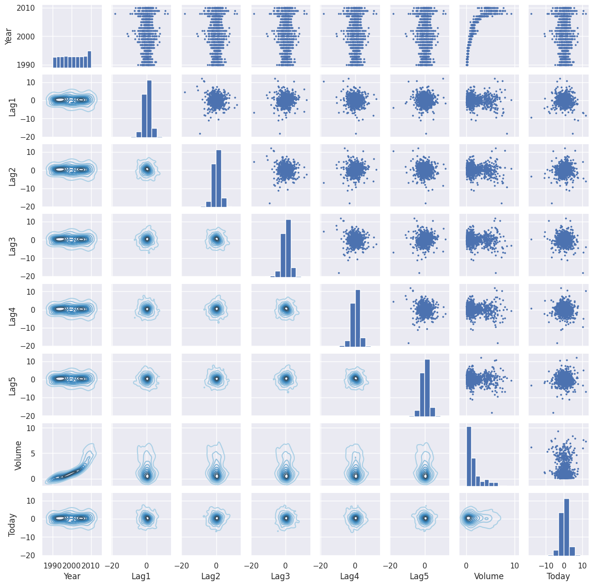
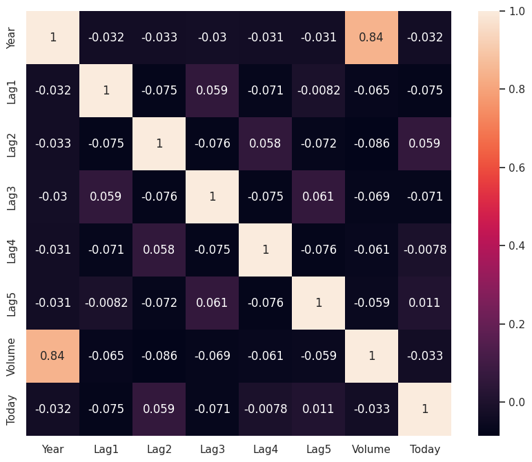
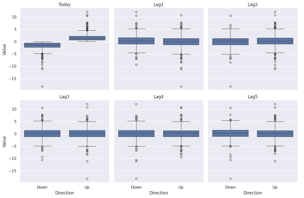
From the plots above we can see that there aren’t any prominant relationships in the data aside from Volume growing with Year.

# Melt DataFrame to long format
weekly_melt = weekly.melt(id_vars=['Direction'], 
                  value_vars=['Today', 'Lag1', 'Lag2', 'Lag3', 'Lag4', 'Lag5'], 
                  var_name='Lag', 
                  value_name='Value')

# Create box plots for each Lag variable
g = sns.catplot(x='Direction', y='Value', col='Lag', 
                data=weekly_melt, kind='box', 
                col_wrap=3, height=4, aspect=1)
g.set_titles("{col_name}")
plt.show()

(b)

vars = weekly.columns.drop(['Today', 'Year', 'Direction'])
design = MS(vars)

X = design.fit_transform(weekly)
y = weekly['Direction'] == 'Up'

glm = sm.GLM(y, 
            X,
            family=sm.families.Binomial())

results = glm.fit()
summarize(results)

	coef	std err	z	P>|z|
intercept	0.2669	0.086	3.106	0.002
Lag1	-0.0413	0.026	-1.563	0.118
Lag2	0.0584	0.027	2.175	0.030
Lag3	-0.0161	0.027	-0.602	0.547
Lag4	-0.0278	0.026	-1.050	0.294
Lag5	-0.0145	0.026	-0.549	0.583
Volume	-0.0227	0.037	-0.616	0.538

Only Lag2 seems to be statistically significant at a confidence level of 5%.

(c)

probs = results.predict()
probs

array([0.60862494, 0.60103144, 0.58756995, ..., 0.57972297, 0.55091703,
       0.52212163])

labels = np.array(['Down']*1089)
labels[probs>0.5] = "Up"

np.unique(labels, return_counts=True)

(array(['Down', 'Up'], dtype='<U4'), array([102, 987]))

np.unique(weekly['Direction'], return_counts=True)

(array(['Down', 'Up'], dtype=object), array([484, 605]))

confusion_table(labels, weekly['Direction'])

Truth	Down	Up
Predicted
Down	54	48
Up	430	557

(54+ 557)/1089, 605/1089

(0.5610651974288338, 0.5555555555555556)

The fraction of correct predictions is 56.1% which is 6.1% better than random guessing and 0.55% better than the null classifer (always predicting Up).

We can also see from the confusion matrix that our model made 430 type I errors and 48 type II errors.

(d)

weekly90_08 = weekly[weekly['Year'] <= 2008]
weekly90_08.describe()

	Year	Lag1	Lag2	Lag3	Lag4	Lag5	Volume	Today
count	985.000000	985.000000	985.000000	985.000000	985.000000	985.000000	985.000000	985.000000
mean	1999.050761	0.124501	0.127820	0.122884	0.122227	0.120976	1.205973	0.130535
std	5.457286	2.269346	2.269069	2.272617	2.272625	2.274273	1.258204	2.279069
min	1990.000000	-18.195000	-18.195000	-18.195000	-18.195000	-18.195000	0.087465	-18.195000
25%	1994.000000	-1.154000	-1.147000	-1.154000	-1.154000	-1.154000	0.307337	-1.154000
50%	1999.000000	0.231000	0.234000	0.231000	0.230000	0.230000	0.804848	0.231000
75%	2004.000000	1.334000	1.337000	1.337000	1.337000	1.337000	1.515846	1.337000
max	2008.000000	12.026000	12.026000	12.026000	12.026000	12.026000	9.328214	12.026000

weekly09_10 = weekly[weekly['Year'] > 2008]
weekly09_10.describe()

	Year	Lag1	Lag2	Lag3	Lag4	Lag5	Volume	Today
count	104.000000	104.000000	104.000000	104.000000	104.000000	104.000000	104.000000	104.000000
mean	2009.500000	0.397635	0.371365	0.377548	0.369250	0.319058	5.066105	0.333298
std	0.502421	3.068538	3.074725	3.075192	3.073895	3.073650	1.147652	3.003296
min	2009.000000	-7.035000	-7.035000	-7.035000	-7.035000	-7.035000	2.390427	-7.035000
25%	2009.000000	-1.060750	-1.214250	-1.214250	-1.214250	-1.323250	4.234228	-1.060750
50%	2009.500000	0.522000	0.461500	0.522000	0.461500	0.437000	4.850717	0.461500
75%	2010.000000	2.239250	2.239250	2.239250	2.239250	2.204250	5.793837	2.204250
max	2010.000000	10.707000	10.707000	10.707000	10.707000	10.707000	7.963276	10.707000

design = MS(['Lag2'])

X = design.fit_transform(weekly90_08)
y = weekly90_08['Direction'] == 'Up'

glm = sm.GLM(y, 
            X,
            family=sm.families.Binomial())

results = glm.fit()
summarize(results)

	coef	std err	z	P>|z|
intercept	0.2033	0.064	3.162	0.002
Lag2	0.0581	0.029	2.024	0.043

X = design.fit_transform(weekly09_10)
probs = results.predict(X)
probs[:10]

985    0.526129
986    0.644736
987    0.486216
988    0.485200
989    0.519767
990    0.540125
991    0.623348
992    0.480993
993    0.451220
994    0.484881
dtype: float64

len(weekly09_10)

104

labels = np.array(['Down']*104)
labels[probs>0.5] = "Up"
confusion_table(labels, weekly09_10['Direction'])

Truth	Down	Up
Predicted
Down	9	5
Up	34	56

(9+56)/104, 61/104

(0.625, 0.5865384615384616)

The fraction of correct predictions is 62.5% which is 12.5% better than random guessing and 3.8% better than the null classifer (always predicting Up).

(e) Since we’ll end up using the same code to fit all the models on the same data I’ll create a function to make that easier:

def fit_and_test(model):
    design = MS(['Lag2'], intercept=False)

    X_train = design.fit_transform(weekly90_08)
    X_test = design.fit_transform(weekly09_10)
    L_train = weekly90_08['Direction']
    L_test = weekly09_10['Direction']

    mdl = model

    mdl = mdl.fit(X_train, L_train)
    
    pred = mdl.predict(X_test)
    return confusion_table(pred, L_test)

Using LDA:

lda = LDA(store_covariance=True)
fit_and_test(lda)

Truth	Down	Up
Predicted
Down	9	5
Up	34	56

(9+56)/(104)

0.625

The fraction of correct predictions is 62.5% which is 12.5% better than random guessing. We can also see that this resulted in the exact same confusion matrix as the Logistic Regression.

(f) Using QDA:

qda = QDA(store_covariance=True)
fit_and_test(qda)

Truth	Down	Up
Predicted
Down	0	0
Up	43	61

61/104

0.5865384615384616

We can see that the QDA model here is equivalent to always predicting Up hence it has the same error rate as the null classifer .

(g) Using KNN with K = 1:

knn = KNeighborsClassifier(n_neighbors=1)
fit_and_test(knn)

Truth	Down	Up
Predicted
Down	22	32
Up	21	29

(22+29)/104

0.49038461538461536

The fraction of correct predictions is 49% which is even worse than random guessing here and much worse than the null classifer.

(h) Using Naive Bayes:

nb = GaussianNB()
fit_and_test(nb)

Truth	Down	Up
Predicted
Down	0	0
Up	43	61

We can see that the Naive Bayes model here is equivalent to always predicting Up hence it has the same error rate as the null classifer and QDA.

(i) LDA and Logistic Regression seem to provide the best predictions with an accuracy of 62.5%.

(j) We’ll try a few different combinations of predictors, transformations, and interactions for each of the methods.

We’ll start by making a slight modification to the function we defined above.

def fit_and_test(modelspec, model):
    """ 
    Takes a ModelSpec for the weekly dataset and a model and trains it on data from 1990 to 2008, 
    then tests it on the data from 2009 to 2010 and returns the fraction of correct predictions and a confusion 
    matrix for the given model and testing.
    """
    design = modelspec

    X_train = design.fit_transform(weekly90_08)
    X_test = design.fit_transform(weekly09_10)
    L_train = weekly90_08['Direction']
    L_test = weekly09_10['Direction']

    mdl = model

    mdl = mdl.fit(X_train, L_train)
    
    pred = mdl.predict(X_test)
    conf_mat = confusion_table(pred, L_test)
    
    print(model.__repr__())
    print(f'fraction of correct predictions: {(conf_mat.iloc[0, 0] + conf_mat.iloc[1, 1])/len(pred):.3f}')
    return conf_mat

modelspec = MS(['Lag2', 'Lag5', 'Lag3',  ('Lag2', 'Lag5'), ('Lag5', 'Lag3')])
fit_and_test(modelspec, LogisticRegression())

LogisticRegression()
fraction of correct predictions: 0.606

Truth	Down	Up
Predicted
Down	9	7
Up	34	54

modelspec = MS(['Lag2', 'Volume',  ('Lag2', 'Volume')])
fit_and_test(modelspec, LogisticRegression())

LogisticRegression()
fraction of correct predictions: 0.529

Truth	Down	Up
Predicted
Down	19	25
Up	24	36

modelspec = MS(['Lag2', 'Lag5', 'Lag3',  ('Lag2', 'Lag5'), ('Lag5', 'Lag3')], intercept=False)
for model in [LDA(), QDA(), GaussianNB()]:
    print(fit_and_test(modelspec, model))
    print()

LinearDiscriminantAnalysis()
fraction of correct predictions: 0.615
Truth      Down  Up
Predicted          
Down          9   6
Up           34  55

QuadraticDiscriminantAnalysis()
fraction of correct predictions: 0.538
Truth      Down  Up
Predicted          
Down         11  16
Up           32  45

GaussianNB()
fraction of correct predictions: 0.529
Truth      Down  Up
Predicted          
Down         10  16
Up           33  45

modelspec = MS(['Lag1', 'Lag2', 'Lag5',  ('Lag1', 'Lag2'), ('Lag5', 'Lag2')], intercept=False)
for model in [LDA(), QDA(), GaussianNB()]:
    print(fit_and_test(modelspec, model))
    print()

LinearDiscriminantAnalysis()
fraction of correct predictions: 0.567
Truth      Down  Up
Predicted          
Down          8  10
Up           35  51

QuadraticDiscriminantAnalysis()
fraction of correct predictions: 0.538
Truth      Down  Up
Predicted          
Down         12  17
Up           31  44

GaussianNB()
fraction of correct predictions: 0.529
Truth      Down  Up
Predicted          
Down          8  14
Up           35  47

Looking at all the combinations of variables and models above we can see that not many get close to LDA and LR’s accuracy score of 62.5% when fit on Lag2. Closest score we had was LDA fit on Lag2, Lag5, Lag3, (Lag2 x Lag5), (Lag5 x Lag3) with an accuracy of 61.5%.

modelspec = MS(['Lag2'], intercept=False)
for k in range(1, 31):
    print(fit_and_test(modelspec, KNeighborsClassifier(n_neighbors=k)))
    print()

KNeighborsClassifier(n_neighbors=1)
fraction of correct predictions: 0.490
Truth      Down  Up
Predicted          
Down         22  32
Up           21  29

KNeighborsClassifier(n_neighbors=2)
fraction of correct predictions: 0.462
Truth      Down  Up
Predicted          
Down         31  44
Up           12  17

KNeighborsClassifier(n_neighbors=3)
fraction of correct predictions: 0.558
Truth      Down  Up
Predicted          
Down         16  19
Up           27  42

KNeighborsClassifier(n_neighbors=4)
fraction of correct predictions: 0.577
Truth      Down  Up
Predicted          
Down         26  27
Up           17  34

KNeighborsClassifier()
fraction of correct predictions: 0.538
Truth      Down  Up
Predicted          
Down         16  21
Up           27  40

KNeighborsClassifier(n_neighbors=6)
fraction of correct predictions: 0.510
Truth      Down  Up
Predicted          
Down         20  28
Up           23  33

KNeighborsClassifier(n_neighbors=7)
fraction of correct predictions: 0.548
Truth      Down  Up
Predicted          
Down         16  20
Up           27  41

KNeighborsClassifier(n_neighbors=8)
fraction of correct predictions: 0.548
Truth      Down  Up
Predicted          
Down         21  25
Up           22  36

KNeighborsClassifier(n_neighbors=9)
fraction of correct predictions: 0.558
Truth      Down  Up
Predicted          
Down         17  20
Up           26  41

KNeighborsClassifier(n_neighbors=10)
fraction of correct predictions: 0.567
Truth      Down  Up
Predicted          
Down         22  24
Up           21  37

KNeighborsClassifier(n_neighbors=11)
fraction of correct predictions: 0.567
Truth      Down  Up
Predicted          
Down         19  21
Up           24  40

KNeighborsClassifier(n_neighbors=12)
fraction of correct predictions: 0.567
Truth      Down  Up
Predicted          
Down         23  25
Up           20  36

KNeighborsClassifier(n_neighbors=13)
fraction of correct predictions: 0.596
Truth      Down  Up
Predicted          
Down         20  19
Up           23  42

KNeighborsClassifier(n_neighbors=14)
fraction of correct predictions: 0.567
Truth      Down  Up
Predicted          
Down         21  23
Up           22  38

KNeighborsClassifier(n_neighbors=15)
fraction of correct predictions: 0.587
Truth      Down  Up
Predicted          
Down         20  20
Up           23  41

KNeighborsClassifier(n_neighbors=16)
fraction of correct predictions: 0.577
Truth      Down  Up
Predicted          
Down         21  22
Up           22  39

KNeighborsClassifier(n_neighbors=17)
fraction of correct predictions: 0.596
Truth      Down  Up
Predicted          
Down         21  20
Up           22  41

KNeighborsClassifier(n_neighbors=18)
fraction of correct predictions: 0.587
Truth      Down  Up
Predicted          
Down         22  22
Up           21  39

KNeighborsClassifier(n_neighbors=19)
fraction of correct predictions: 0.567
Truth      Down  Up
Predicted          
Down         19  21
Up           24  40

KNeighborsClassifier(n_neighbors=20)
fraction of correct predictions: 0.596
Truth      Down  Up
Predicted          
Down         23  22
Up           20  39

KNeighborsClassifier(n_neighbors=21)
fraction of correct predictions: 0.558
Truth      Down  Up
Predicted          
Down         19  22
Up           24  39

KNeighborsClassifier(n_neighbors=22)
fraction of correct predictions: 0.596
Truth      Down  Up
Predicted          
Down         23  22
Up           20  39

KNeighborsClassifier(n_neighbors=23)
fraction of correct predictions: 0.567
Truth      Down  Up
Predicted          
Down         20  22
Up           23  39

KNeighborsClassifier(n_neighbors=24)
fraction of correct predictions: 0.558
Truth      Down  Up
Predicted          
Down         22  25
Up           21  36

KNeighborsClassifier(n_neighbors=25)
fraction of correct predictions: 0.548
Truth      Down  Up
Predicted          
Down         19  23
Up           24  38

KNeighborsClassifier(n_neighbors=26)
fraction of correct predictions: 0.538
Truth      Down  Up
Predicted          
Down         23  28
Up           20  33

KNeighborsClassifier(n_neighbors=27)
fraction of correct predictions: 0.529
Truth      Down  Up
Predicted          
Down         18  24
Up           25  37

KNeighborsClassifier(n_neighbors=28)
fraction of correct predictions: 0.529
Truth      Down  Up
Predicted          
Down         21  27
Up           22  34

KNeighborsClassifier(n_neighbors=29)
fraction of correct predictions: 0.548
Truth      Down  Up
Predicted          
Down         19  23
Up           24  38

KNeighborsClassifier(n_neighbors=30)
fraction of correct predictions: 0.529
Truth      Down  Up
Predicted          
Down         21  27
Up           22  34

Trying the KNN classifier using the Lag2 variable and neighbors from 1 to 30, we can see that it yielded the highest accuracy of 59.6% for values of K = 13, 17, 20, 22.

Q14.

auto = load_data('Auto')
auto.head()

	mpg	cylinders	displacement	horsepower	weight	acceleration	year	origin
name
chevrolet chevelle malibu	18.0	8	307.0	130	3504	12.0	70	1
buick skylark 320	15.0	8	350.0	165	3693	11.5	70	1
plymouth satellite	18.0	8	318.0	150	3436	11.0	70	1
amc rebel sst	16.0	8	304.0	150	3433	12.0	70	1
ford torino	17.0	8	302.0	140	3449	10.5	70	1

auto.info()

<class 'pandas.core.frame.DataFrame'>
Index: 392 entries, chevrolet chevelle malibu to chevy s-10
Data columns (total 8 columns):
 #   Column        Non-Null Count  Dtype  
---  ------        --------------  -----  
 0   mpg           392 non-null    float64
 1   cylinders     392 non-null    int64  
 2   displacement  392 non-null    float64
 3   horsepower    392 non-null    int64  
 4   weight        392 non-null    int64  
 5   acceleration  392 non-null    float64
 6   year          392 non-null    int64  
 7   origin        392 non-null    int64  
dtypes: float64(3), int64(5)
memory usage: 27.6+ KB

auto.describe()

	mpg	cylinders	displacement	horsepower	weight	acceleration	year	origin
count	392.000000	392.000000	392.000000	392.000000	392.000000	392.000000	392.000000	392.000000
mean	23.445918	5.471939	194.411990	104.469388	2977.584184	15.541327	75.979592	1.576531
std	7.805007	1.705783	104.644004	38.491160	849.402560	2.758864	3.683737	0.805518
min	9.000000	3.000000	68.000000	46.000000	1613.000000	8.000000	70.000000	1.000000
25%	17.000000	4.000000	105.000000	75.000000	2225.250000	13.775000	73.000000	1.000000
50%	22.750000	4.000000	151.000000	93.500000	2803.500000	15.500000	76.000000	1.000000
75%	29.000000	8.000000	275.750000	126.000000	3614.750000	17.025000	79.000000	2.000000
max	46.600000	8.000000	455.000000	230.000000	5140.000000	24.800000	82.000000	3.000000

(a)

mpg01 = auto['mpg'] > auto['mpg'].median()
mpg01

name
chevrolet chevelle malibu    False
buick skylark 320            False
plymouth satellite           False
amc rebel sst                False
ford torino                  False
                             ...  
ford mustang gl               True
vw pickup                     True
dodge rampage                 True
ford ranger                   True
chevy s-10                    True
Name: mpg, Length: 392, dtype: bool

auto['mpg01'] = mpg01.astype(int)
auto.head()

	mpg	cylinders	displacement	horsepower	weight	acceleration	year	origin	mpg01
name
chevrolet chevelle malibu	18.0	8	307.0	130	3504	12.0	70	1	0
buick skylark 320	15.0	8	350.0	165	3693	11.5	70	1	0
plymouth satellite	18.0	8	318.0	150	3436	11.0	70	1	0
amc rebel sst	16.0	8	304.0	150	3433	12.0	70	1	0
ford torino	17.0	8	302.0	140	3449	10.5	70	1	0

(b)

g = sns.PairGrid(auto)
g.map_upper(plt.scatter, s=3, alpha=0.7)
g.map_diag(plt.hist, alpha=0.6)

def lower_plots(x, y, **kwargs):
    if y.name in ['mpg01', 'origin']: 
        num_colors_needed = y.nunique()
        sns.boxplot(x=x, y=y, orient='h', hue=y, palette=sns.color_palette('Blues_d', n_colors=num_colors_needed), **kwargs)  # Horizontal boxplot
    else:
        sns.kdeplot(x=x, y=y, cmap='Blues_d', **kwargs)  # KDE plot

g.map_lower(lower_plots)
g.figure.set_size_inches(12, 12);

plt.figure(figsize=(10, 10))
sns.heatmap(auto.corr(), annot=True, square=True);

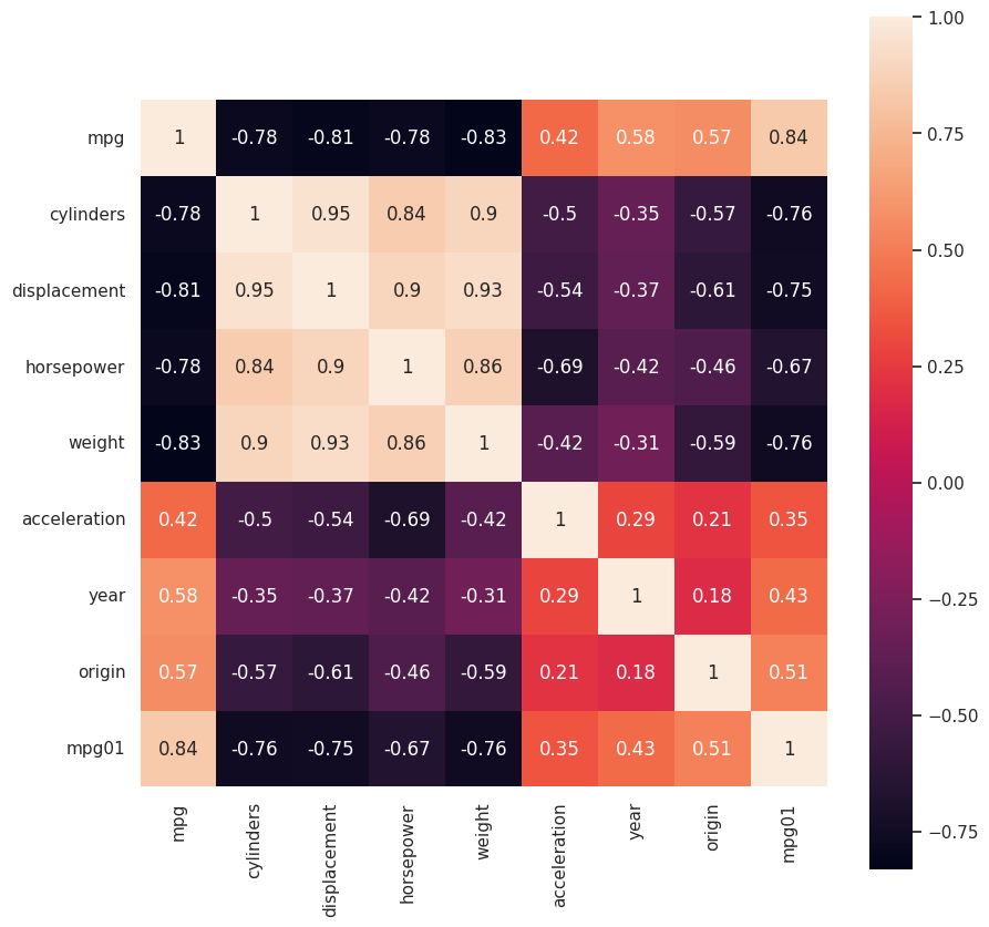
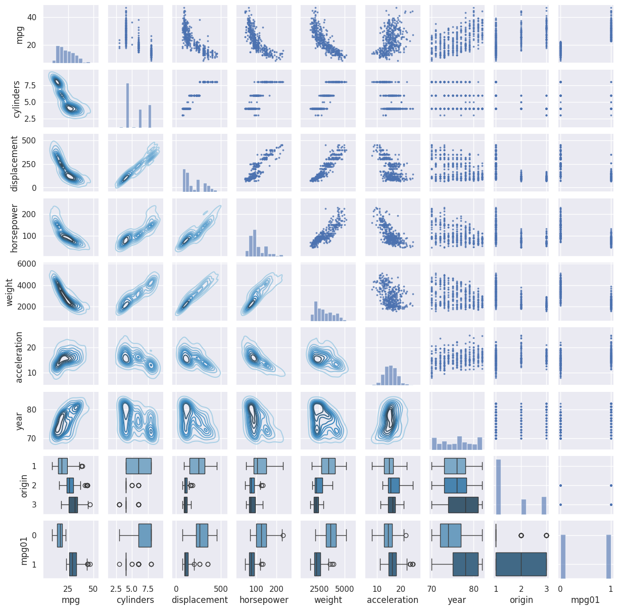
Looking at the heatmap and the plots above we can see that many of them have some sort of relationship with mpg01, the most useful for predicting mpg01 would likely be features like cylinders, displacement, horsepower, weight.

(c)

X = auto[['cylinders', 'displacement', 'horsepower', 'weight']]
y = auto['mpg01']

X_train, X_test, y_train, y_test = train_test_split(X, y, test_size=0.3, random_state=1)

(d) LDA:

lda = LDA()
lda.fit(X_train, y_train)
lda_pred = lda.predict(X_test)
lda_pred

array([1, 1, 1, 1, 1, 1, 1, 0, 1, 1, 0, 1, 0, 1, 1, 0, 1, 1, 0, 0, 1, 0,
       0, 0, 0, 0, 1, 0, 0, 1, 0, 1, 0, 0, 0, 0, 0, 0, 1, 1, 0, 0, 1, 0,
       0, 0, 0, 1, 0, 0, 0, 0, 1, 1, 1, 0, 1, 1, 1, 1, 0, 1, 1, 0, 0, 0,
       1, 0, 1, 0, 1, 0, 0, 1, 1, 1, 0, 0, 0, 1, 0, 1, 1, 1, 0, 0, 1, 1,
       1, 0, 1, 0, 0, 0, 0, 1, 0, 1, 0, 0, 1, 1, 0, 1, 1, 1, 0, 1, 0, 0,
       1, 0, 1, 1, 0, 1, 0, 0])

Defining a quick function to get the error rate from a confusion matrix.

def get_error_rate(conf_mat):
    return (conf_mat.iloc[0, 1] + conf_mat.iloc[1, 0])/conf_mat.sum().sum()

conf_mat = confusion_table(lda_pred, y_test)
conf_mat

Truth	0	1
Predicted
0	58	3
1	7	50

get_error_rate(conf_mat)

0.0847457627118644

The test error rate for LDA is 8.5%.

(e) QDA:

qda = QDA()
qda.fit(X_train, y_train)
qda_pred = qda.predict(X_test)
qda_pred

array([1, 1, 1, 1, 1, 1, 1, 0, 1, 1, 0, 1, 0, 1, 1, 0, 1, 1, 0, 0, 1, 0,
       0, 0, 0, 0, 1, 0, 0, 1, 0, 1, 0, 0, 0, 0, 0, 0, 1, 1, 0, 0, 0, 0,
       0, 0, 0, 1, 0, 0, 0, 0, 1, 1, 1, 0, 0, 0, 1, 1, 0, 1, 1, 0, 0, 0,
       0, 0, 1, 0, 1, 0, 0, 1, 1, 1, 0, 0, 0, 1, 0, 1, 1, 1, 0, 0, 1, 1,
       1, 0, 1, 0, 0, 0, 0, 0, 0, 1, 0, 0, 1, 1, 0, 1, 1, 1, 0, 1, 0, 0,
       1, 0, 1, 1, 0, 1, 0, 0])

conf_mat = confusion_table(qda_pred, y_test)
conf_mat

Truth	0	1
Predicted
0	61	5
1	4	48

get_error_rate(conf_mat)

0.07627118644067797

The test error rate for QDA is 7.6%.

(f)

lr = LogisticRegression()
lr.fit(X_train, y_train)
lr_pred = lr.predict(X_test)
lr_pred

array([1, 1, 1, 1, 1, 1, 1, 0, 1, 1, 0, 1, 0, 1, 1, 0, 1, 1, 0, 0, 1, 0,
       0, 0, 0, 0, 1, 0, 0, 1, 0, 1, 0, 0, 0, 0, 0, 0, 1, 1, 0, 0, 0, 0,
       0, 0, 0, 1, 0, 0, 0, 0, 1, 1, 1, 0, 0, 1, 1, 1, 0, 1, 1, 0, 0, 0,
       1, 0, 1, 0, 1, 0, 0, 1, 1, 1, 0, 0, 0, 1, 0, 1, 1, 1, 0, 0, 1, 1,
       1, 0, 1, 0, 0, 0, 0, 0, 0, 1, 0, 0, 1, 1, 0, 1, 1, 1, 0, 1, 0, 0,
       1, 1, 1, 1, 0, 1, 0, 0])

conf_mat = confusion_table(lr_pred, y_test)
conf_mat

Truth	0	1
Predicted
0	59	4
1	6	49

get_error_rate(conf_mat)

0.0847457627118644

The test error rate for Logistic Regression is 8.5%.

(g) Naive Bayes:

nb = GaussianNB()
nb.fit(X_train, y_train)
nb_pred = nb.predict(X_test)
nb_pred

array([1, 1, 1, 1, 1, 1, 1, 0, 1, 1, 0, 1, 0, 1, 1, 0, 1, 1, 0, 0, 1, 0,
       0, 0, 0, 0, 1, 0, 0, 1, 0, 1, 0, 0, 0, 0, 0, 0, 1, 1, 0, 0, 0, 0,
       0, 0, 0, 1, 0, 0, 0, 0, 1, 1, 1, 0, 0, 0, 1, 1, 0, 1, 1, 0, 0, 0,
       1, 0, 1, 0, 1, 0, 0, 1, 1, 1, 0, 0, 0, 1, 0, 1, 1, 1, 0, 0, 1, 1,
       1, 0, 1, 0, 0, 0, 0, 0, 0, 1, 0, 0, 1, 1, 0, 1, 1, 1, 0, 1, 0, 0,
       1, 0, 1, 1, 0, 1, 0, 0])

conf_mat = confusion_table(nb_pred, y_test)
conf_mat

Truth	0	1
Predicted
0	60	5
1	5	48

get_error_rate(conf_mat)

0.0847457627118644

The test error rate for Naive Bayes is 8.5%.

(h) KNN:

For this we’ll use StandardScaler since KNN uses distances between points to make predictions.

scaler = StandardScaler(with_mean=True,
                        with_std=True,
                        copy=True)

X = auto[['cylinders', 'displacement', 'horsepower', 'weight']]
y = auto['mpg01']


X_std = scaler.fit_transform(X)
feature_std = pd.DataFrame(
                 X_std,
                 columns=X.columns);
feature_std.std()

cylinders       1.001278
displacement    1.001278
horsepower      1.001278
weight          1.001278
dtype: float64

X_train_std, X_test_std, y_train_std, y_test_std  = train_test_split(np.asarray(feature_std), y, test_size=0.3,random_state=1)

error_rate = {}
for k in range(1, 200):
    knn = KNeighborsClassifier(n_neighbors=k)

    knn.fit(X_train_std, y_train_std)
    knn_pred = knn.predict(X_test_std)
    conf_mat = confusion_table(knn_pred, y_test_std)
    error_rate[k] = get_error_rate(conf_mat)

plt.plot(error_rate.keys(), error_rate.values())
plt.xlabel('K')
plt.ylabel('Error Rate');
k_min = min(error_rate, key=error_rate.get)
k_min, error_rate[k_min]

(8, 0.059322033898305086)

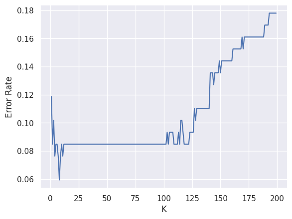
The best value for K in the KNN classifier for this dataset is 8 which resulted in the minimal error rate of 5.93%.

Q15.

(a)

def Power():
    """ Prints the result of raising 2 to the 3rd power """
    print(2 ** 3)

Power()

8

(b)

def Power2(x, a):
    """ Prints the result of raising x to the power a """
    print(x ** a)

Power2(3, 8)

6561

(c)

Power2(10, 3) 
Power2(8, 17)
Power2(131, 3)

1000
2251799813685248
2248091

(d)

def Power3(x, a):
    """ returns the result of raising x to the power a """
    result = x ** a
    return result

(e)

x = np.arange(1, 11)
y = Power3(x, 2)

plt.plot (x, y)

plt.title('$f(x) = x^2$')
plt.xlabel('x-axis')
plt.ylabel('y-axis');
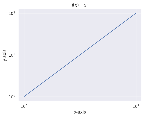
plt.xscale('log')
plt.yscale('log')

plt.plot (x, y)

plt.title('$f(x) = x^2$')
plt.xlabel('x-axis')
plt.ylabel('y-axis');
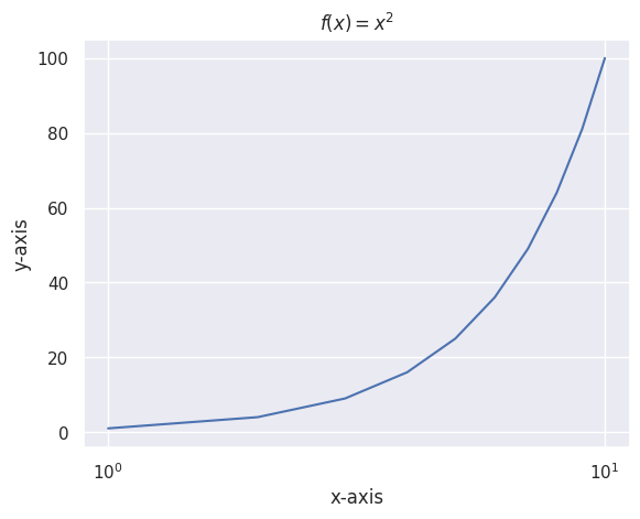
plt.xscale('log')

plt.plot (x, y)

plt.title('$f(x) = x^2$')
plt.xlabel('x-axis')
plt.ylabel('y-axis');
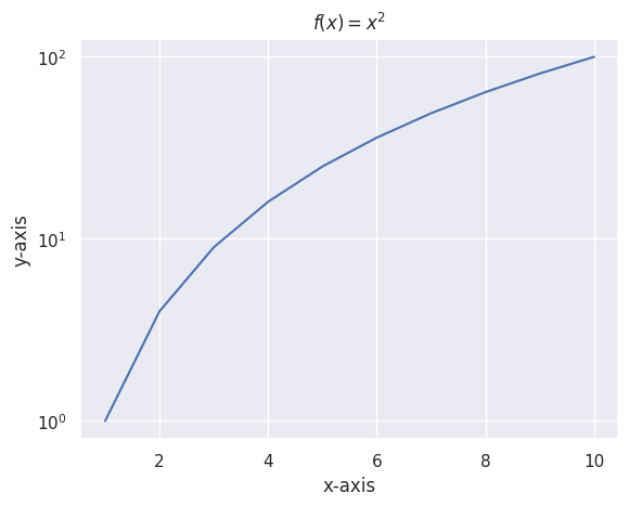
plt.yscale('log')

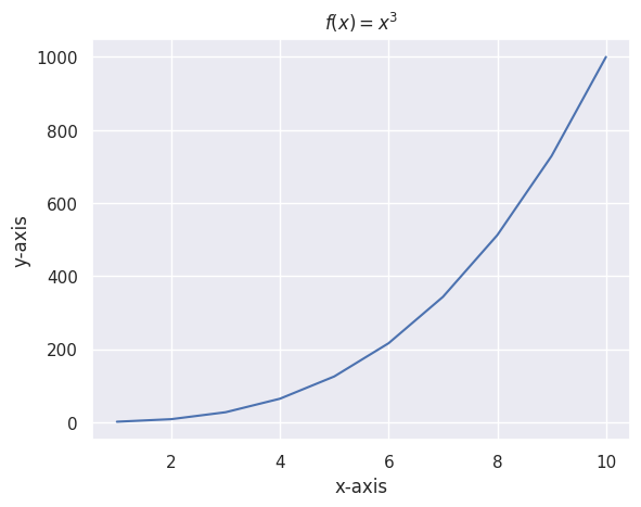
(f)

def PlotPower(x, a):
    y = Power3(x, a)
    plt.plot (x, y)

    plt.title(f'$f(x) = x^{a}$')
    plt.xlabel('x-axis')
    plt.ylabel('y-axis');

PlotPower(np.arange(1, 11), 3)

Q16.

The same as Q14.

boston = load_data('Boston')
boston.head()

	crim	zn	indus	chas	nox	rm	age	dis	rad	tax	ptratio	lstat	medv
0	0.00632	18.0	2.31	0	0.538	6.575	65.2	4.0900	1	296	15.3	4.98	24.0
1	0.02731	0.0	7.07	0	0.469	6.421	78.9	4.9671	2	242	17.8	9.14	21.6
2	0.02729	0.0	7.07	0	0.469	7.185	61.1	4.9671	2	242	17.8	4.03	34.7
3	0.03237	0.0	2.18	0	0.458	6.998	45.8	6.0622	3	222	18.7	2.94	33.4
4	0.06905	0.0	2.18	0	0.458	7.147	54.2	6.0622	3	222	18.7	5.33	36.2

boston.info()

<class 'pandas.core.frame.DataFrame'>
RangeIndex: 506 entries, 0 to 505
Data columns (total 13 columns):
 #   Column   Non-Null Count  Dtype  
---  ------   --------------  -----  
 0   crim     506 non-null    float64
 1   zn       506 non-null    float64
 2   indus    506 non-null    float64
 3   chas     506 non-null    int64  
 4   nox      506 non-null    float64
 5   rm       506 non-null    float64
 6   age      506 non-null    float64
 7   dis      506 non-null    float64
 8   rad      506 non-null    int64  
 9   tax      506 non-null    int64  
 10  ptratio  506 non-null    float64
 11  lstat    506 non-null    float64
 12  medv     506 non-null    float64
dtypes: float64(10), int64(3)
memory usage: 51.5 KB

boston.describe()

	crim	zn	indus	chas	nox	rm	age	dis	rad	tax	ptratio	lstat	medv
count	506.000000	506.000000	506.000000	506.000000	506.000000	506.000000	506.000000	506.000000	506.000000	506.000000	506.000000	506.000000	506.000000
mean	3.613524	11.363636	11.136779	0.069170	0.554695	6.284634	68.574901	3.795043	9.549407	408.237154	18.455534	12.653063	22.532806
std	8.601545	23.322453	6.860353	0.253994	0.115878	0.702617	28.148861	2.105710	8.707259	168.537116	2.164946	7.141062	9.197104
min	0.006320	0.000000	0.460000	0.000000	0.385000	3.561000	2.900000	1.129600	1.000000	187.000000	12.600000	1.730000	5.000000
25%	0.082045	0.000000	5.190000	0.000000	0.449000	5.885500	45.025000	2.100175	4.000000	279.000000	17.400000	6.950000	17.025000
50%	0.256510	0.000000	9.690000	0.000000	0.538000	6.208500	77.500000	3.207450	5.000000	330.000000	19.050000	11.360000	21.200000
75%	3.677083	12.500000	18.100000	0.000000	0.624000	6.623500	94.075000	5.188425	24.000000	666.000000	20.200000	16.955000	25.000000
max	88.976200	100.000000	27.740000	1.000000	0.871000	8.780000	100.000000	12.126500	24.000000	711.000000	22.000000	37.970000	50.000000

First we’ll create a variable crim01 which indicates whether the crime rate is below (0) or above (1) the median.

boston['crim01'] = (boston['crim'] > boston['crim'].median()).astype(int)
boston['crim01'].sample(5, random_state=1)

307    0
343    0
47     0
67     0
362    1
Name: crim01, dtype: int64

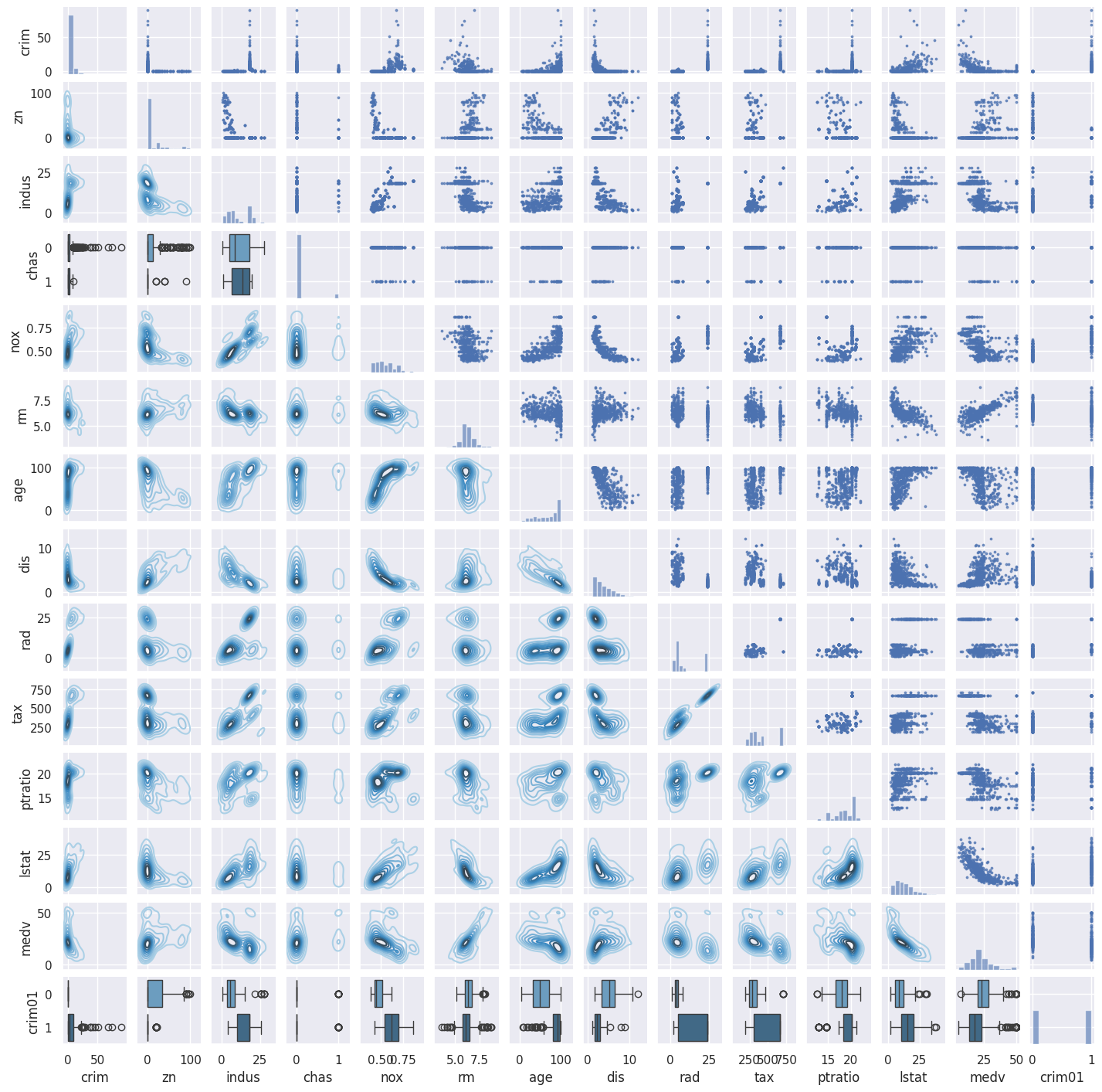
Now we’ll explore the data to see what features would be useful in predicting crim01.

g = sns.PairGrid(boston)
g.map_upper(plt.scatter, s=3, alpha=0.7)
g.map_diag(plt.hist, alpha=0.6)

def lower_plots(x, y, **kwargs):
    if y.name in ['crim01', 'chas']: 
        num_colors_needed = y.nunique()
        sns.boxplot(x=x, y=y, orient='h', hue=y, palette=sns.color_palette('Blues_d', n_colors=num_colors_needed), **kwargs)  # Horizontal boxplot
    else:
        sns.kdeplot(x=x, y=y, cmap='Blues_d', **kwargs)  # KDE plot

g.map_lower(lower_plots)
g.figure.set_size_inches(14, 14);

plt.figure(figsize=(14, 14))
sns.heatmap(boston.corr(), annot=True);

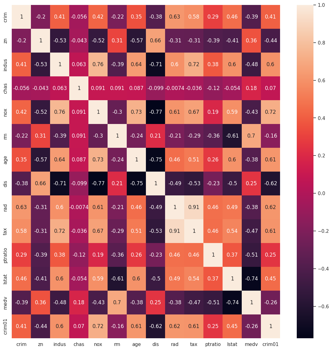
Looking at the heatmap and the plots, I decided to use the variables indus, nox, age, dis, rad, tax because seem to have strong relationships with crim01.

X = boston[['indus', 'nox', 'age', 'dis', 'rad', 'tax']]
y = boston['crim01']

def fit_and_get_error_rate(model, X, y):
    
    X_train, X_test, y_train, y_test = train_test_split(X, y, test_size=0.3, random_state=1)
    
    mdl = model
    
    mdl.fit(X_train, y_train)
    pred = mdl.predict(X_test)
    conf_mat = confusion_table(pred, y_test)
    return get_error_rate(conf_mat)

Using the function above on the 4 models to fit them and get their error rates:

for model in [LDA(), QDA(), LogisticRegression(max_iter=1000), GaussianNB()]:
    print(f'{model.__str__().split("(")[0]}: {fit_and_get_error_rate(model, X, y)}\n')

LinearDiscriminantAnalysis: 0.17763157894736842

QuadraticDiscriminantAnalysis: 0.125

LogisticRegression: 0.17763157894736842

GaussianNB: 0.19078947368421054

We can see the test error rate for each of the models and see that QDA performed the best here with a test error rate of 12.5%.

Now to fit the KNN classifier we’ll start by standardizing the data.

scaler = StandardScaler(with_mean=True,
                        with_std=True,
                        copy=True)

X_std = scaler.fit_transform(X)

feature_std = pd.DataFrame(
                 X_std,
                 columns=X.columns);

feature_std.std()

indus    1.00099
nox      1.00099
age      1.00099
dis      1.00099
rad      1.00099
tax      1.00099
dtype: float64

X_train_std, X_test_std, y_train_std, y_test_std  = train_test_split(feature_std, y, test_size=0.4,random_state=1)

error_rate = {}
for k in range(1, 200):
    knn = KNeighborsClassifier(n_neighbors=k)

    knn.fit(X_train_std, y_train_std)
    knn_pred = knn.predict(X_test_std)
    conf_mat = confusion_table(knn_pred, y_test_std)
    error_rate[k] = get_error_rate(conf_mat)

plt.plot(error_rate.keys(), error_rate.values())
plt.xlabel('K')
plt.ylabel('Error Rate');
k_min = min(error_rate, key=error_rate.get)
k_min, error_rate[k_min]

(6, 0.06403940886699508)

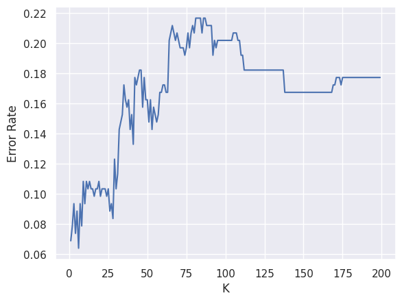
K = 6 seems to be the best value for the KNN classifier with a test error rate of 6.4%.