


Ch6: Linear Model Selection and Regularization#
import matplotlib.pyplot as plt
import numpy as np
import pandas as pd
import seaborn as sns

sns.set_theme()

%matplotlib inline
from functools import partial

import sklearn.linear_model as skl
import sklearn.model_selection as skm
from ISLP import load_data
from ISLP.models import ModelSpec as MS
from sklearn.preprocessing import StandardScaler
from statsmodels.api import OLS
from ISLP.models import Stepwise, sklearn_selected
from sklearn.cross_decomposition import PLSRegression
from sklearn.decomposition import PCA
from sklearn.pipeline import Pipeline
Conceptual#
Q1.#
(a)
Best Subset selection would have the lowest training RSS for any given k, because it goes through the entire search space of \(2^p\) possible models, while forward and backward stepwise perform a guided search through the search space potentially missing combinations of predictors with lower training RSS where the best model with \(k\) predictors might not be a subset of the best model with \(k+1\) predictors.
(b)
There’s not enough information to answer this question as any of the models could have the lowest test RSS depending on the validation method and training and test sets.
(c)
i. True
ii. True
iii. False
iv. False
v. False
Q2.#
(a)
(iii) is the correct statement. The lasso is less flexible than least squares since it has an additional constraint namely the \(\ell_1\) norm of the coefficients has to be less than a certain budget \(s\), which results in an increase in bias that is offset by a decrease in variance.
(b)
(iii) is the correct statement. Ridge regression is less flexible than least squares since it has an additional constraint namely the \(\ell_2\) norm of the coefficients has to be less than a certain budget \(s\), which results in an increase in bias that is offset by a decrease in variance.
(c)
(ii) is the correct statement. Non-linear models are more flexible than least squares, which means they have lower bias and higher variance, Hence they give better predictions when the increase in variance is less than the decrease in bias.
Q3.#
(a)
iv. Steadily decrease.
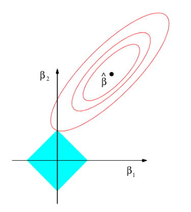
When \(s = 0\) the constraint region would be a dot at the origin, meaning all coefficients are zero with a training RSS equivalent to the null model. As \(s\) increases the size of the diamond constraint region increases including smaller values of RSS until eventually including the least squares estimates \(\hat\beta\) which is the smallest RSS value it can get to.
(b)
ii. Decrease initially, and then eventually start increasing in a U shape.
As we increase the value of \(s\) the flexibility of the model increases resulting in a decrease in bias and an increase in variance. For low values of \(s\) the model would have a high bias and for high values of \(s\) the model would have high variance, so its lowest test RSS would be at a point in the middle that minimizes the test RSS.
(c)
iii. Steadily increase.
As increasing the value of \(s\) increases flexibility hence increasing variance.
(d)
iv. Steadily decrease.
As increasing the value of \(s\) increases flexibility hence decreasing bias.
(e)
(v) Remains constant.
Because it’s the error term that captures variability not included in our model (noise inherent in the data).
Q4.#
(a)
iii. Steadily increase.
At \(\lambda = 0\) the coefficient estimates are equivalent to the least squares estimates, and as \(\lambda\) increases the flexibility of the model decreases, resulting in a greater training RSS, until it becomes equivalent to the training RSS of the null model at \(\lambda = \infty\).
(b)
ii. Decrease initially, then eventually start increasing in a U shape.
At small values of \(\lambda\) where the flexibility is high, the model has high variance and low bias. As \(\lambda\) increases the flexibility of the model decreases, reducing the variance and increasing the bias which results in a lower value of the test RSS. Eventually the flexibility gets too low and the model becomes too rigid to fit the data due to the high bias and low variance resulting in an increase in the test RSS.
(c)
iv. Steadily decrease.
As \(\lambda\) increases the flexibility of the model decreases, resulting in a decrease in variance.
(d)
iii. Steadily increase.
As \(\lambda\) increases the flexibility of the model decreases, resulting in an increase in bias.
(e)
(v) Remains constant.
Because it’s the error term that captures variability not included in our model (noise inherent in the data).
Q5.#
(a) The ridge regression optimization problem takes the form:
Find the coefficients \(\hat\beta^R\) that minimize the following quantity:
Expanding the equation above:
Substituting for \(\hat\beta = 0,\quad x_{11} = x_{12},\quad x_{21} = x_{22},\quad x_{21} = - x_{11}\) and \(y_2 = -y_1\):
We finally get to:
(b) To minimize the equation above we’ll set its derivatives with respect to \(\hat\beta_0, \hat\beta_1\) to \(0\):
By symmetry we can see that \(\hat\beta_1 = \hat\beta_2\):
(c) The lasso regression optimization problem takes the form:
Find the coefficients \(\hat\beta^L\) that minimize the following quantity:
Expanding the equation above:
Substituting for \(\hat\beta = 0,\quad x_{11} = x_{12},\quad x_{21} = x_{22},\quad x_{21} = - x_{11}\) and \(y_2 = -y_1\):
We finally get to:
(d) Starting with the equation we got from (c) and simplifying using \(\hat\beta_1 + \hat\beta_2 = c\):
For a fixed value of \(c\), the minimal value of \(|\hat\beta_1| + |\hat\beta_2|\) is \(|c|\) which is achieved when \(|\hat\beta_1|\) and \(|\hat\beta_2|\) have the same sign so the problem reduces to:
The optimal \(c^*\) depends on \(y_1, x_{11}, \lambda\) and we can see from above that there are infinitely many pairs (\(\hat\beta_1, \hat\beta_2\)) that satisfy \(\hat\beta_1 + \hat\beta_2 = c^*\) given that \(c^*\neq0\) which is why the solutions aren’t unique in this setting.
This is a better answer to this question I found online.
https://www.mathstat.dal.ca/~aarms2014/StatLearn/assignments/A3sol_2.pdf
Q6.#
(a) Starting with (6.12):
For \(\lambda = 5\) and \(y_1 = 24\) (chosen arbitrarly and greater than zero):
def f(y1, lamda, beta1):
    return (y1 - beta1)**2 + lamda * beta1**2

lamda = 5
y1 = 24
beta1 = np.linspace(0, 10, 1000)
y_hat =  f(y1, lamda, beta1)

plt.plot(beta1, y_hat);
plt.xlabel('$\\beta_1$')
plt.ylabel(f'$({y1} - \\beta_1)^2 + {lamda} \\beta_1^2$')
plt.scatter(beta1[np.argmin(y_hat)], np.min(y_hat), color='r');
beta1[np.argmin(y_hat)]
4.004004004004004
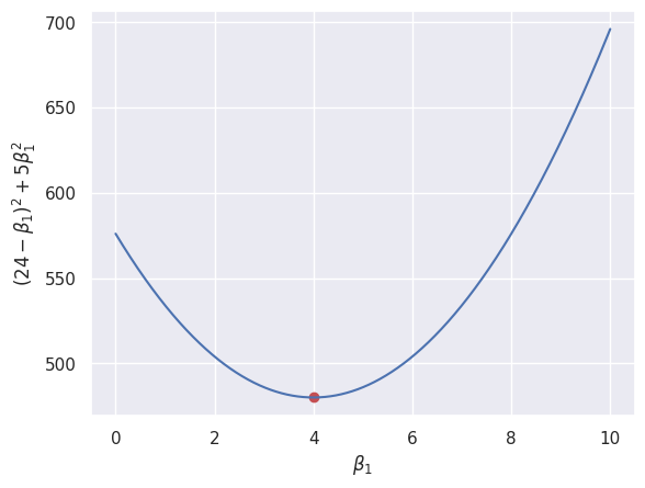
Now using the formula \((6.14)\):
y1/(1+lamda)
4.0
We can see that the result from the equation above agrees with the plot and that \(\hat\beta_1 = 4\) minimizes the equation.
(b) Starting with equation \((6.13)\):
To prove that the equation below (6.15) solves (6.13), we’ll have to confirm that the plots agree on the minimum value picked from each case.
For \(\lambda = 5\) and \(y_1 = 24\) (chosen arbitrarly to match case 1):
lamda = 5
y1 = 24

y1 > lamda/2
True
def f(y1, lamda, beta1):
    return (y1 - beta1)**2 + lamda * np.abs(beta1)

beta1 = np.linspace(-50, 100, 1000)
y_hat =  f(y1, lamda, beta1)

plt.plot(beta1, y_hat);
plt.xlabel('$\\beta_1$')
plt.ylabel(f'$({y1} - \\beta_1)^2 + {lamda} |\\beta_1|$')
plt.scatter(beta1[np.argmin(y_hat)], np.min(y_hat), color='r');
beta1[np.argmin(y_hat)]
21.471471471471475
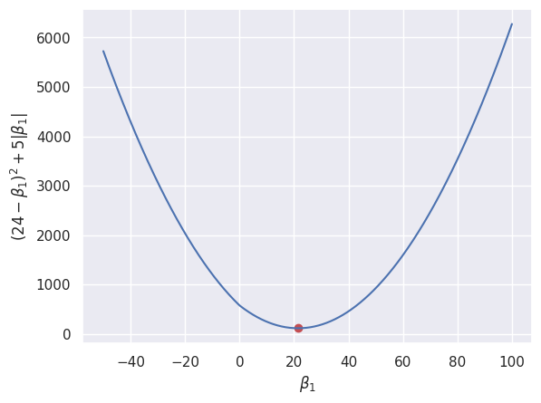
Using (6.15) and since \(y_1 > \lambda/2\):
y1 - lamda/2
21.5
We can see that both results agree and that \(\hat\beta_1 = 21.5\) minimizes the equation.
For case 2, we choose the values of \(\lambda = 10\) and \(y_1 = -40\):
lamda = 10
y1 = -40

y1 < -lamda/2
True
def f(y1, lamda, beta1):
    return (y1 - beta1)**2 + lamda * np.abs(beta1)

beta1 = np.linspace(-120, 100, 1000)
y_hat =  f(y1, lamda, beta1)

plt.plot(beta1, y_hat);
plt.xlabel('$\\beta_1$')
plt.ylabel(f'$({y1} - \\beta_1)^2 + {lamda} |\\beta_1|$')
plt.scatter(beta1[np.argmin(y_hat)], np.min(y_hat), color='r')
plt.text(beta1[np.argmin(y_hat)]-20, 1200, f"({beta1[np.argmin(y_hat)]:.2f}, {np.min(y_hat):.2f})", fontdict={"fontsize":10});
beta1[np.argmin(y_hat)]
-34.994994994995
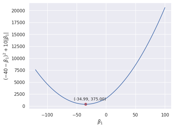
For case 2:
y1 + lamda/2
-35.0
We can see that it agrees with the plot and \(\hat\beta_1^L = -35\) minimizes the equation.
For case 3 we choose \(y_1 = 2\) and \(\lambda = 4\):
y1 = 2
lamda = 4

np.abs(y1) <= lamda/2
True
def f(y1, lamda, beta1):
    return (y1 - beta1)**2 + lamda * np.abs(beta1)

beta1 = np.linspace(-20, 20, 1000)
y_hat =  f(y1, lamda, beta1)

plt.plot(beta1, y_hat);
plt.xlabel('$\\beta_1$')
plt.ylabel(f'$({y1} - \\beta_1)^2 + {lamda} |\\beta_1|$')
plt.scatter(beta1[np.argmin(y_hat)], np.min(y_hat), color='r')
plt.text(beta1[np.argmin(y_hat)]-2, 30, f"({beta1[np.argmin(y_hat)]:.2f}, {np.min(y_hat):.2f})", fontdict={"fontsize":10});
beta1[np.argmin(y_hat)]
0.020020020020020013
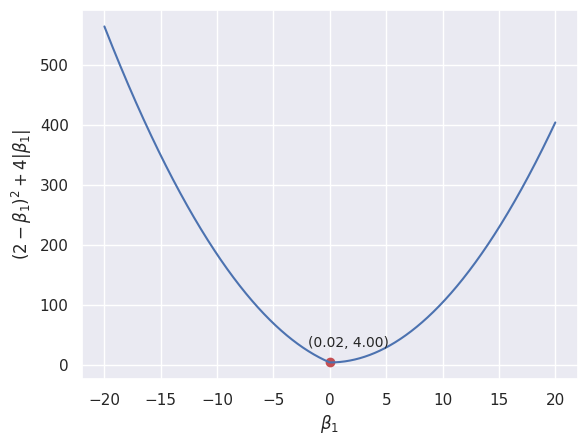
For case 3:
From the plot we can see that the minima of the plot is at \(0\) which agrees with the coefficient picked by (6.15) case 3.
Q7.#
(a) We can see that \(y_i\) is normally distributed with mean \(\beta_0 + \sum_{j=1}^{p} x_{ij} \beta_{j}\) and variance \(\sigma^2\):
Hence:
And since all \(y_i\) are independant and identically distributed the likelihood would be the product of all their probability distributions.
(b) Since all \(\beta_i\) are \(i.i.d\) with a double-exponential distribution with mean \(0\) and common scale parameter \(b\) as their prior:
Then:
The posterior is:
(c) First we’ll find the mode \(\hat\beta_{MAP}\) by maximizing probability density function above, we’ll do that by taking its logarithm:
To maximize the logarithm above we only need to consider terms that vary with \(\beta\):
We can see that the terms are similar to the lasso problem, with a least squares sum on the left and an L1 penalty on the right. The difference here is that we’re trying to maximize a negative quantity whereas in the lasso we try to minimize a positive quantity.
Since:
We can simply rewrite the problem as:
This is equivalent to the lasso estimate with \(\lambda = \frac{2\sigma^2}{b}\):
Expanding the expression above:
(d) Since all \(\beta_i\) are \(i.i.d\) with a normal distribution with a mean \(0\) and variance \(c\):
Then:
The posterior for \( \beta \) is:
(e) We’ll follow the same steps in (C) to find the mode \(\hat\beta_{MAP}\):
Since:
We can simply rewrite the problem as:
This is equivalent to the ridge regression estimate with \(\lambda = \sigma^2/c\).
Expanding the expression above:
Since \(p(\beta | X, Y)\) is a product of two multivariate normal distributions then it’s also a multivariate normal distribution, which means its mode equals its mean resulting in:
Applied#
Q8.#
(a)
rng = np.random.default_rng(1)
x = rng.normal(size=100)
eps = rng.normal(size=100)
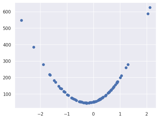
(b) We’ll simply pick the constants to be:
Now we’ll generate the response vector \(Y\) according to the model:
b0 = 50
b1 = 44
b2 = 97
b3 = 5

y = b0 + b1 * x + b2 * x**2 + b3 * x**3 + eps
y[:10]
array([ 76.34534441, 155.26730418,  75.18533933, 146.99222541,
       174.27288033,  89.79538712,  52.69118937, 107.79282114,
        80.92941577,  71.34962123])
plt.scatter(x, y);
(c)
def nCp(sigma2, estimator, X, Y):
    "Negative Cp statistic"
    n, p = X.shape
    Yhat = estimator.predict(X)
    RSS = np.sum((Y - Yhat)**2)
    return -(RSS + 2 * p * sigma2) / n
First we’ll estimate the variance \(\sigma^2\) so we can use the \(C_p\) metric, we’ll do that by fitting a model with all the predictors \(X, X^2, ..., X^{10}\).
df = pd.DataFrame({f'x^{i}':x**i for i in range(1, 11)})
df['y'] = y
df.head()
| x^1 | x^2 | x^3 | x^4 | x^5 | x^6 | x^7 | x^8 | x^9 | x^10 | y | |
|---|---|---|---|---|---|---|---|---|---|---|---|
| 0 | 0.345584 | 0.119428 | 0.041273 | 0.014263 | 0.004929 | 0.001703 | 0.000589 | 0.000203 | 0.000070 | 0.000024 | 76.345344 |
| 1 | 0.821618 | 0.675056 | 0.554639 | 0.455701 | 0.374412 | 0.307624 | 0.252749 | 0.207663 | 0.170620 | 0.140185 | 155.267304 |
| 2 | 0.330437 | 0.109189 | 0.036080 | 0.011922 | 0.003940 | 0.001302 | 0.000430 | 0.000142 | 0.000047 | 0.000016 | 75.185339 |
| 3 | -1.303157 | 1.698219 | -2.213046 | 2.883947 | -3.758236 | 4.897573 | -6.382308 | 8.317150 | -10.838554 | 14.124341 | 146.992225 |
| 4 | 0.905356 | 0.819669 | 0.742092 | 0.671858 | 0.608270 | 0.550701 | 0.498580 | 0.451393 | 0.408671 | 0.369993 | 174.272880 |
design = MS(df.columns.drop('y')).fit(df)
Y = np.array(df['y'])
# we drop the intercept here because the fitting process later adds an intercept
X = design.transform(df).drop('intercept', axis=1)
sigma2 = OLS(Y,X).fit().scale
sigma2
814.8803706928072
neg_Cp = partial(nCp, sigma2)
Now we’ll fit the model using forward stepwise selection.
strategy = Stepwise.first_peak(design,
                               direction='forward',
                               max_terms=len(design.terms))

model_forward = sklearn_selected(OLS,
                              strategy,
                              scoring=neg_Cp)

model_forward.fit(X, Y)
model_forward.selected_state_
('x^1', 'x^2', 'x^3')
model_forward.results_.summary()
| Dep. Variable: | y | R-squared: | 1.000 |
|---|---|---|---|
| Model: | OLS | Adj. R-squared: | 1.000 |
| Method: | Least Squares | F-statistic: | 3.597e+05 |
| Date: | Mon, 24 Mar 2025 | Prob (F-statistic): | 2.85e-194 |
| Time: | 10:19:04 | Log-Likelihood: | -140.47 |
| No. Observations: | 100 | AIC: | 288.9 |
| Df Residuals: | 96 | BIC: | 299.4 |
| Df Model: | 3 | ||
| Covariance Type: | nonrobust |
| coef | std err | t | P>|t| | [0.025 | 0.975] | |
|---|---|---|---|---|---|---|
| intercept | 49.9428 | 0.120 | 416.437 | 0.000 | 49.705 | 50.181 |
| x^1 | 44.1146 | 0.187 | 235.313 | 0.000 | 43.742 | 44.487 |
| x^2 | 96.9529 | 0.099 | 979.102 | 0.000 | 96.756 | 97.149 |
| x^3 | 4.9357 | 0.060 | 82.151 | 0.000 | 4.816 | 5.055 |
| Omnibus: | 0.845 | Durbin-Watson: | 2.199 |
|---|---|---|---|
| Prob(Omnibus): | 0.655 | Jarque-Bera (JB): | 0.392 |
| Skew: | 0.052 | Prob(JB): | 0.822 |
| Kurtosis: | 3.289 | Cond. No. | 5.95 |
Notes:
[1] Standard Errors assume that the covariance matrix of the errors is correctly specified.
The model obtained according to \(C_p\) is:
And the coefficients are:
We can see that the estimated coefficients are pretty close to the ones in the true underlying model.
(d) Using backwards stepwise:
strategy = Stepwise.first_peak(design,
                               direction='backwards',
                               max_terms=len(design.terms))

model_backwards = sklearn_selected(OLS,
                              strategy,
                              scoring=neg_Cp)

model_backwards.fit(X, Y)
model_backwards.selected_state_
('x^1', 'x^2', 'x^3')
model_backwards.results_.summary()
| Dep. Variable: | y | R-squared: | 1.000 |
|---|---|---|---|
| Model: | OLS | Adj. R-squared: | 1.000 |
| Method: | Least Squares | F-statistic: | 3.597e+05 |
| Date: | Mon, 24 Mar 2025 | Prob (F-statistic): | 2.85e-194 |
| Time: | 10:19:04 | Log-Likelihood: | -140.47 |
| No. Observations: | 100 | AIC: | 288.9 |
| Df Residuals: | 96 | BIC: | 299.4 |
| Df Model: | 3 | ||
| Covariance Type: | nonrobust |
| coef | std err | t | P>|t| | [0.025 | 0.975] | |
|---|---|---|---|---|---|---|
| intercept | 49.9428 | 0.120 | 416.437 | 0.000 | 49.705 | 50.181 |
| x^1 | 44.1146 | 0.187 | 235.313 | 0.000 | 43.742 | 44.487 |
| x^2 | 96.9529 | 0.099 | 979.102 | 0.000 | 96.756 | 97.149 |
| x^3 | 4.9357 | 0.060 | 82.151 | 0.000 | 4.816 | 5.055 |
| Omnibus: | 0.845 | Durbin-Watson: | 2.199 |
|---|---|---|---|
| Prob(Omnibus): | 0.655 | Jarque-Bera (JB): | 0.392 |
| Skew: | 0.052 | Prob(JB): | 0.822 |
| Kurtosis: | 3.289 | Cond. No. | 5.95 |
Notes:
[1] Standard Errors assume that the covariance matrix of the errors is correctly specified.
We got the same exact model obtained from (c):
(e)
K = 5

outer_valid = skm.ShuffleSplit(n_splits=1,
                               test_size=0.25,
                               random_state=1)

inner_kfold = skm.KFold(n_splits=K,
               shuffle=True,
               random_state=2)

scaler = StandardScaler()

lassoCV = skl.ElasticNetCV(l1_ratio=1,
                           cv=inner_kfold)

pipeCV = Pipeline([('scaler', scaler),
                ('lasso', lassoCV)])

results = skm.cross_validate(pipeCV,
                             X,
                             Y,
                             cv=outer_valid,
                             scoring='neg_mean_squared_error')
-results['test_score']
array([0.95807935])
pipeCV.fit(X, Y)
Pipeline(steps=[('scaler', StandardScaler()),
                ('lasso',
                 ElasticNetCV(cv=KFold(n_splits=5, random_state=2, shuffle=True),
                              l1_ratio=1))])
In a Jupyter environment, please rerun this cell to show the HTML representation or trust the notebook. On GitHub, the HTML representation is unable to render, please try loading this page with nbviewer.org.
Pipeline(steps=[('scaler', StandardScaler()),
                ('lasso',
                 ElasticNetCV(cv=KFold(n_splits=5, random_state=2, shuffle=True),
l1_ratio=1))])StandardScaler()
ElasticNetCV(cv=KFold(n_splits=5, random_state=2, shuffle=True), l1_ratio=1)
tuned_lasso = pipeCV.named_steps['lasso']
tuned_lasso.coef_
array([ 3.73534163e+01,  1.14483615e+02,  1.43824335e+01,  0.00000000e+00,
        0.00000000e+00,  2.05614973e-01, -0.00000000e+00,  8.29412867e-02,
       -0.00000000e+00,  5.53145176e-02])
tuned_lasso.alpha_
0.09434150271628827
The optimal value of \(\lambda\) that minimizes the CV error is \(9.567\times10^{-9}\).
Now we’ll plot the CV error against \(-\log(\lambda)\). Most of this data is stored in the tuned lasso model.
lassoCV_fig, ax = plt.subplots(figsize=(8,8))
ax.errorbar(-np.log(tuned_lasso.alphas_),
            tuned_lasso.mse_path_.mean(1),
            yerr=tuned_lasso.mse_path_.std(1) / np.sqrt(K))
ax.axvline(-np.log(tuned_lasso.alpha_), c='k', ls='--')
ax.set_xlabel('$-\log(\lambda)$', fontsize=20)
ax.set_ylabel('Cross-validated MSE', fontsize=20);
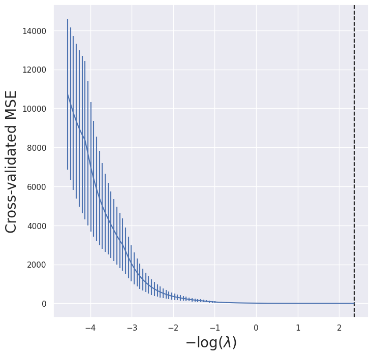
The CV MSE seems to stabilize for very small values of \(\lambda\) (approaching zero). Looking at the graph one would wonder what results you get at \(\lambda=0\) (OLS fit with all predictors) but that’s not part of the question.
tuned_lasso.intercept_
115.50547867740701
tuned_lasso.coef_
array([ 3.73534163e+01,  1.14483615e+02,  1.43824335e+01,  0.00000000e+00,
        0.00000000e+00,  2.05614973e-01, -0.00000000e+00,  8.29412867e-02,
       -0.00000000e+00,  5.53145176e-02])
These are the values of the resulting coefficients:
We can rescale them to understand what they mean better.
scaler = pipeCV.named_steps['scaler']
tuned_lasso.coef_/ scaler.scale_
array([ 4.38648593e+01,  9.66391029e+01,  4.97622121e+00,  0.00000000e+00,
        0.00000000e+00,  4.78954023e-03, -0.00000000e+00,  2.76075239e-04,
       -0.00000000e+00,  2.55588074e-05])
And rescale the intercept seperately.
tuned_lasso.intercept_ - np.dot(tuned_lasso.coef_, scaler.mean_/scaler.scale_)
50.109058104632226
Note that the estimated coefficients \(\hat\beta_1, \hat\beta_2, \hat\beta_3\) are very close to the true underlying coefficients, while the other coefficients mistakenly included by the model have values close to \(0\).
(f)
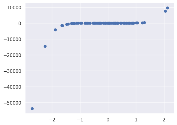
b0 = 23
b7 = 50
y = b0 + b7 * x**7 + eps
df = pd.DataFrame({f'x^{i}':x**i for i in range(1, 11)})
df['y'] = y
df.head()
| x^1 | x^2 | x^3 | x^4 | x^5 | x^6 | x^7 | x^8 | x^9 | x^10 | y | |
|---|---|---|---|---|---|---|---|---|---|---|---|
| 0 | 0.345584 | 0.119428 | 0.041273 | 0.014263 | 0.004929 | 0.001703 | 0.000589 | 0.000203 | 0.000070 | 0.000024 | 22.378153 |
| 1 | 0.821618 | 0.675056 | 0.554639 | 0.455701 | 0.374412 | 0.307624 | 0.252749 | 0.207663 | 0.170620 | 0.140185 | 36.499915 |
| 2 | 0.330437 | 0.109189 | 0.036080 | 0.011922 | 0.003940 | 0.001302 | 0.000430 | 0.000142 | 0.000047 | 0.000016 | 22.895915 |
| 3 | -1.303157 | 1.698219 | -2.213046 | 2.883947 | -3.758236 | 4.897573 | -6.382308 | 8.317150 | -10.838554 | 14.124341 | -295.446225 |
| 4 | 0.905356 | 0.819669 | 0.742092 | 0.671858 | 0.608270 | 0.550701 | 0.498580 | 0.451393 | 0.408671 | 0.369993 | 49.147866 |
plt.scatter(x, y);
design = MS(df.columns.drop('y')).fit(df)
Y = np.array(df['y'])
X = design.transform(df).drop('intercept', axis=1)
sigma2 = OLS(Y,X).fit().scale
sigma2
173.27265731949643
neg_Cp = partial(nCp, sigma2)
strategy = Stepwise.first_peak(design,
                               direction='forward',
                               max_terms=len(design.terms))

model_forward = sklearn_selected(OLS,
                              strategy,
                              scoring=neg_Cp)

model_forward.fit(X, Y)
model_forward.selected_state_
('x^7',)
model_forward.results_.summary()
| Dep. Variable: | y | R-squared: | 1.000 |
|---|---|---|---|
| Model: | OLS | Adj. R-squared: | 1.000 |
| Method: | Least Squares | F-statistic: | 3.364e+09 |
| Date: | Mon, 24 Mar 2025 | Prob (F-statistic): | 0.00 |
| Time: | 10:19:05 | Log-Likelihood: | -139.12 |
| No. Observations: | 100 | AIC: | 282.2 |
| Df Residuals: | 98 | BIC: | 287.4 |
| Df Model: | 1 | ||
| Covariance Type: | nonrobust |
| coef | std err | t | P>|t| | [0.025 | 0.975] | |
|---|---|---|---|---|---|---|
| intercept | 22.9048 | 0.099 | 231.740 | 0.000 | 22.709 | 23.101 |
| x^7 | 49.9983 | 0.001 | 5.8e+04 | 0.000 | 49.997 | 50.000 |
| Omnibus: | 0.958 | Durbin-Watson: | 2.208 |
|---|---|---|---|
| Prob(Omnibus): | 0.619 | Jarque-Bera (JB): | 0.479 |
| Skew: | -0.035 | Prob(JB): | 0.787 |
| Kurtosis: | 3.332 | Cond. No. | 115. |
Notes:
[1] Standard Errors assume that the covariance matrix of the errors is correctly specified.
Forward stepwise selection was able to correctly identify the significance of the intercept and \(X^7\) and made very good estimates for them.
Fitting the lasso model:
scaler = StandardScaler()

K = 5

kfold = skm.KFold(n_splits=K,
               shuffle=True,
               random_state=2)

lassoCV = skl.ElasticNetCV(l1_ratio=1,
                           cv=kfold)

pipeCV = Pipeline([('scaler', scaler),
                ('lasso', lassoCV)])
pipeCV.fit(X, Y)
Pipeline(steps=[('scaler', StandardScaler()),
                ('lasso',
                 ElasticNetCV(cv=KFold(n_splits=5, random_state=2, shuffle=True),
                              l1_ratio=1))])
In a Jupyter environment, please rerun this cell to show the HTML representation or trust the notebook. On GitHub, the HTML representation is unable to render, please try loading this page with nbviewer.org.
Pipeline(steps=[('scaler', StandardScaler()),
                ('lasso',
                 ElasticNetCV(cv=KFold(n_splits=5, random_state=2, shuffle=True),
l1_ratio=1))])StandardScaler()
ElasticNetCV(cv=KFold(n_splits=5, random_state=2, shuffle=True), l1_ratio=1)
tuned_lasso = pipeCV.named_steps['lasso']
tuned_lasso.coef_
array([ -23.83668   ,    0.        ,    0.        ,   -0.        ,
        884.14226819,   -0.        , 3554.24953   ,   -0.        ,
       1292.65572729,   -0.        ])
We can see that the lasso selected the predictors \(X, X^5, X^7, X^9\) with the coefficients \(-23.84, 884.14, 3554.25, 1292.66\) respectively.
We can also rescale them using the following code to understand them better.
scaler = pipeCV.named_steps['scaler']
tuned_lasso.coef_/ scaler.scale_
array([-27.99188718,   0.        ,   0.        ,  -0.        ,
        52.25920473,  -0.        ,  31.18606038,  -0.        ,
         1.5992205 ,  -0.        ])
tuned_lasso.intercept_ - np.dot(tuned_lasso.coef_, scaler.mean_ / scaler.scale_)
29.426020977326743
We can see that the lasso ended up with a pretty weird model containing various predictors not originally in the true underlying model.
Forward stepwise did a lot better than the lasso here.
Q9.#
college = load_data('College')
college.head()
| Private | Apps | Accept | Enroll | Top10perc | Top25perc | F.Undergrad | P.Undergrad | Outstate | Room.Board | Books | Personal | PhD | Terminal | S.F.Ratio | perc.alumni | Expend | Grad.Rate | |
|---|---|---|---|---|---|---|---|---|---|---|---|---|---|---|---|---|---|---|
| 0 | Yes | 1660 | 1232 | 721 | 23 | 52 | 2885 | 537 | 7440 | 3300 | 450 | 2200 | 70 | 78 | 18.1 | 12 | 7041 | 60 |
| 1 | Yes | 2186 | 1924 | 512 | 16 | 29 | 2683 | 1227 | 12280 | 6450 | 750 | 1500 | 29 | 30 | 12.2 | 16 | 10527 | 56 |
| 2 | Yes | 1428 | 1097 | 336 | 22 | 50 | 1036 | 99 | 11250 | 3750 | 400 | 1165 | 53 | 66 | 12.9 | 30 | 8735 | 54 |
| 3 | Yes | 417 | 349 | 137 | 60 | 89 | 510 | 63 | 12960 | 5450 | 450 | 875 | 92 | 97 | 7.7 | 37 | 19016 | 59 |
| 4 | Yes | 193 | 146 | 55 | 16 | 44 | 249 | 869 | 7560 | 4120 | 800 | 1500 | 76 | 72 | 11.9 | 2 | 10922 | 15 |
college.info()
<class 'pandas.core.frame.DataFrame'>
RangeIndex: 777 entries, 0 to 776
Data columns (total 18 columns):
 #   Column       Non-Null Count  Dtype
---  ------       --------------  -----
 0   Private      777 non-null    category
 1   Apps         777 non-null    int64
 2   Accept       777 non-null    int64
 3   Enroll       777 non-null    int64
 4   Top10perc    777 non-null    int64
 5   Top25perc    777 non-null    int64
 6   F.Undergrad  777 non-null    int64
 7   P.Undergrad  777 non-null    int64
 8   Outstate     777 non-null    int64
 9   Room.Board   777 non-null    int64
 10  Books        777 non-null    int64
 11  Personal     777 non-null    int64
 12  PhD          777 non-null    int64
 13  Terminal     777 non-null    int64
 14  S.F.Ratio    777 non-null    float64
 15  perc.alumni  777 non-null    int64
 16  Expend       777 non-null    int64
 17  Grad.Rate    777 non-null    int64
dtypes: category(1), float64(1), int64(16)
memory usage: 104.2 KB
college.describe(include='all')
| Private | Apps | Accept | Enroll | Top10perc | Top25perc | F.Undergrad | P.Undergrad | Outstate | Room.Board | Books | Personal | PhD | Terminal | S.F.Ratio | perc.alumni | Expend | Grad.Rate | |
|---|---|---|---|---|---|---|---|---|---|---|---|---|---|---|---|---|---|---|
| count | 777 | 777.000000 | 777.000000 | 777.000000 | 777.000000 | 777.000000 | 777.000000 | 777.000000 | 777.000000 | 777.000000 | 777.000000 | 777.000000 | 777.000000 | 777.000000 | 777.000000 | 777.000000 | 777.000000 | 777.00000 |
| unique | 2 | NaN | NaN | NaN | NaN | NaN | NaN | NaN | NaN | NaN | NaN | NaN | NaN | NaN | NaN | NaN | NaN | NaN |
| top | Yes | NaN | NaN | NaN | NaN | NaN | NaN | NaN | NaN | NaN | NaN | NaN | NaN | NaN | NaN | NaN | NaN | NaN |
| freq | 565 | NaN | NaN | NaN | NaN | NaN | NaN | NaN | NaN | NaN | NaN | NaN | NaN | NaN | NaN | NaN | NaN | NaN |
| mean | NaN | 3001.638353 | 2018.804376 | 779.972973 | 27.558559 | 55.796654 | 3699.907336 | 855.298584 | 10440.669241 | 4357.526384 | 549.380952 | 1340.642214 | 72.660232 | 79.702703 | 14.089704 | 22.743887 | 9660.171171 | 65.46332 |
| std | NaN | 3870.201484 | 2451.113971 | 929.176190 | 17.640364 | 19.804778 | 4850.420531 | 1522.431887 | 4023.016484 | 1096.696416 | 165.105360 | 677.071454 | 16.328155 | 14.722359 | 3.958349 | 12.391801 | 5221.768440 | 17.17771 |
| min | NaN | 81.000000 | 72.000000 | 35.000000 | 1.000000 | 9.000000 | 139.000000 | 1.000000 | 2340.000000 | 1780.000000 | 96.000000 | 250.000000 | 8.000000 | 24.000000 | 2.500000 | 0.000000 | 3186.000000 | 10.00000 |
| 25% | NaN | 776.000000 | 604.000000 | 242.000000 | 15.000000 | 41.000000 | 992.000000 | 95.000000 | 7320.000000 | 3597.000000 | 470.000000 | 850.000000 | 62.000000 | 71.000000 | 11.500000 | 13.000000 | 6751.000000 | 53.00000 |
| 50% | NaN | 1558.000000 | 1110.000000 | 434.000000 | 23.000000 | 54.000000 | 1707.000000 | 353.000000 | 9990.000000 | 4200.000000 | 500.000000 | 1200.000000 | 75.000000 | 82.000000 | 13.600000 | 21.000000 | 8377.000000 | 65.00000 |
| 75% | NaN | 3624.000000 | 2424.000000 | 902.000000 | 35.000000 | 69.000000 | 4005.000000 | 967.000000 | 12925.000000 | 5050.000000 | 600.000000 | 1700.000000 | 85.000000 | 92.000000 | 16.500000 | 31.000000 | 10830.000000 | 78.00000 |
| max | NaN | 48094.000000 | 26330.000000 | 6392.000000 | 96.000000 | 100.000000 | 31643.000000 | 21836.000000 | 21700.000000 | 8124.000000 | 2340.000000 | 6800.000000 | 103.000000 | 100.000000 | 39.800000 | 64.000000 | 56233.000000 | 118.00000 |
(a)
design = MS(college.columns.drop('Apps'))

X = design.fit_transform(college)
y = college['Apps']

X_train, X_test, y_train, y_test = skm.train_test_split(X, y, test_size=0.3, random_state=1)
(b)
results = OLS(y_train, X_train).fit()
pred = results.predict(X_test)
ols_MSE = np.mean((pred - y_test)**2)
ols_MSE
642753.8976528522
We got a test MSE of \(642753.90\).
(c)
X[:5]
| intercept | Private[Yes] | Accept | Enroll | Top10perc | Top25perc | F.Undergrad | P.Undergrad | Outstate | Room.Board | Books | Personal | PhD | Terminal | S.F.Ratio | perc.alumni | Expend | Grad.Rate | |
|---|---|---|---|---|---|---|---|---|---|---|---|---|---|---|---|---|---|---|
| 0 | 1.0 | 1.0 | 1232 | 721 | 23 | 52 | 2885 | 537 | 7440 | 3300 | 450 | 2200 | 70 | 78 | 18.1 | 12 | 7041 | 60 |
| 1 | 1.0 | 1.0 | 1924 | 512 | 16 | 29 | 2683 | 1227 | 12280 | 6450 | 750 | 1500 | 29 | 30 | 12.2 | 16 | 10527 | 56 |
| 2 | 1.0 | 1.0 | 1097 | 336 | 22 | 50 | 1036 | 99 | 11250 | 3750 | 400 | 1165 | 53 | 66 | 12.9 | 30 | 8735 | 54 |
| 3 | 1.0 | 1.0 | 349 | 137 | 60 | 89 | 510 | 63 | 12960 | 5450 | 450 | 875 | 92 | 97 | 7.7 | 37 | 19016 | 59 |
| 4 | 1.0 | 1.0 | 146 | 55 | 16 | 44 | 249 | 869 | 7560 | 4120 | 800 | 1500 | 76 | 72 | 11.9 | 2 | 10922 | 15 |
We have to drop the intercept when fitting RidgeCV and LassoCV since they add an intercept by default.
X_train = X_train.drop('intercept', axis=1)
X_test = X_test.drop('intercept', axis=1)
K = 5
lambdas = np.linspace(0, 50, 100)

inner_kfold = skm.KFold(n_splits=K,
               shuffle=True,
               random_state=2)

scaler = StandardScaler()

ridgeCV = skl.RidgeCV(alphas=lambdas,
                      cv=inner_kfold)

pipeCV = Pipeline([('scaler', scaler),
                ('ridge', ridgeCV)])

pipeCV.fit(X_train, y_train)
Pipeline(steps=[('scaler', StandardScaler()),
                ('ridge',
                 RidgeCV(alphas=array([ 0.        ,  0.50505051,  1.01010101,  1.51515152,  2.02020202,
        2.52525253,  3.03030303,  3.53535354,  4.04040404,  4.54545455,
        5.05050505,  5.55555556,  6.06060606,  6.56565657,  7.07070707,
        7.57575758,  8.08080808,  8.58585859,  9.09090909,  9.5959596 ,
       10.1010101 , 10.60606061, 11.11111111, 11.61616162, 12.12121212,
       12.62...
       35.35353535, 35.85858586, 36.36363636, 36.86868687, 37.37373737,
       37.87878788, 38.38383838, 38.88888889, 39.39393939, 39.8989899 ,
       40.4040404 , 40.90909091, 41.41414141, 41.91919192, 42.42424242,
       42.92929293, 43.43434343, 43.93939394, 44.44444444, 44.94949495,
       45.45454545, 45.95959596, 46.46464646, 46.96969697, 47.47474747,
       47.97979798, 48.48484848, 48.98989899, 49.49494949, 50.        ]),
                         cv=KFold(n_splits=5, random_state=2, shuffle=True)))])
In a Jupyter environment, please rerun this cell to show the HTML representation or trust the notebook. On GitHub, the HTML representation is unable to render, please try loading this page with nbviewer.org.
Pipeline(steps=[('scaler', StandardScaler()),
                ('ridge',
                 RidgeCV(alphas=array([ 0.        ,  0.50505051,  1.01010101,  1.51515152,  2.02020202,
        2.52525253,  3.03030303,  3.53535354,  4.04040404,  4.54545455,
        5.05050505,  5.55555556,  6.06060606,  6.56565657,  7.07070707,
        7.57575758,  8.08080808,  8.58585859,  9.09090909,  9.5959596 ,
       10.1010101 , 10.60606061, 11.11111111, 11.61616162, 12.12121212,
       12.62...
       35.35353535, 35.85858586, 36.36363636, 36.86868687, 37.37373737,
       37.87878788, 38.38383838, 38.88888889, 39.39393939, 39.8989899 ,
       40.4040404 , 40.90909091, 41.41414141, 41.91919192, 42.42424242,
       42.92929293, 43.43434343, 43.93939394, 44.44444444, 44.94949495,
       45.45454545, 45.95959596, 46.46464646, 46.96969697, 47.47474747,
       47.97979798, 48.48484848, 48.98989899, 49.49494949, 50.        ]),
cv=KFold(n_splits=5, random_state=2, shuffle=True)))])StandardScaler()
RidgeCV(alphas=array([ 0.        ,  0.50505051,  1.01010101,  1.51515152,  2.02020202,
        2.52525253,  3.03030303,  3.53535354,  4.04040404,  4.54545455,
        5.05050505,  5.55555556,  6.06060606,  6.56565657,  7.07070707,
        7.57575758,  8.08080808,  8.58585859,  9.09090909,  9.5959596 ,
       10.1010101 , 10.60606061, 11.11111111, 11.61616162, 12.12121212,
       12.62626263, 13.13131313, 13.63636364, 14.14141414, 14.6464646...
       35.35353535, 35.85858586, 36.36363636, 36.86868687, 37.37373737,
       37.87878788, 38.38383838, 38.88888889, 39.39393939, 39.8989899 ,
       40.4040404 , 40.90909091, 41.41414141, 41.91919192, 42.42424242,
       42.92929293, 43.43434343, 43.93939394, 44.44444444, 44.94949495,
       45.45454545, 45.95959596, 46.46464646, 46.96969697, 47.47474747,
       47.97979798, 48.48484848, 48.98989899, 49.49494949, 50.        ]),
cv=KFold(n_splits=5, random_state=2, shuffle=True))pipeCV.named_steps['ridge'].alpha_
8.080808080808081
pred = pipeCV.predict(X_test)
ridge_MSE = np.mean((pred - y_test)**2)
ridge_MSE
668492.5378936714
pipeCV.named_steps['ridge'].intercept_
3090.7329650092083
pipeCV.named_steps['ridge'].coef_
array([-1.63231511e+02,  3.52552333e+03, -2.50526186e+02,  8.51856420e+02,
       -2.44289738e+02,  1.91467139e+02,  3.96478531e+01, -3.03344785e+02,
        2.02248350e+02, -1.17161850e+01, -2.21112834e-01, -1.39384427e+02,
       -4.20845395e+01,  6.40900697e+01, -2.73971161e+01,  4.45765894e+02,
        1.69484877e+02])
The test MSE obtained for the ridge regression is \(668492.54\).
(d)
K = 5

inner_kfold = skm.KFold(n_splits=K,
               shuffle=True,
               random_state=2)

scaler = StandardScaler()

lassoCV = skl.ElasticNetCV(l1_ratio=1,
                           cv=inner_kfold)

pipeCV = Pipeline([('scaler', scaler),
                ('lasso', lassoCV)])

pipeCV.fit(X_train, y_train)
Pipeline(steps=[('scaler', StandardScaler()),
                ('lasso',
                 ElasticNetCV(cv=KFold(n_splits=5, random_state=2, shuffle=True),
                              l1_ratio=1))])
In a Jupyter environment, please rerun this cell to show the HTML representation or trust the notebook. On GitHub, the HTML representation is unable to render, please try loading this page with nbviewer.org.
Pipeline(steps=[('scaler', StandardScaler()),
                ('lasso',
                 ElasticNetCV(cv=KFold(n_splits=5, random_state=2, shuffle=True),
l1_ratio=1))])StandardScaler()
ElasticNetCV(cv=KFold(n_splits=5, random_state=2, shuffle=True), l1_ratio=1)
tuned_lasso = pipeCV.named_steps['lasso']
tuned_lasso.alpha_
35.25263542775875
pred = pipeCV.predict(X_test)
lasso_MSE = np.mean((pred - y_test)**2)
lasso_MSE
711843.8332488546
The test MSE obtained for the lasso model is \(711843.83\).
tuned_lasso.intercept_
3090.7329650092083
tuned_lasso.coef_
array([-9.79298525e+01,  3.54463084e+03, -0.00000000e+00,  5.57558717e+02,
       -0.00000000e+00,  0.00000000e+00,  0.00000000e+00, -2.03090809e+02,
        1.27406960e+02,  0.00000000e+00,  0.00000000e+00, -8.17549143e+01,
       -2.30633926e+01,  0.00000000e+00, -2.47229901e+00,  3.76424922e+02,
        6.88473000e+01])
sum(tuned_lasso.coef_ != 0)
10
11 out of 18 coefficients had non-zero estimates including the intercept.
(e)
scaler = StandardScaler()
pca = PCA()
linreg = skl.LinearRegression()

pipe = Pipeline([('scaler', scaler),
                 ('pca', pca),
                 ('linreg', linreg)])

param_grid = {'pca__n_components': range(1, 18)}

K = 5

kfold = skm.KFold(n_splits=K,
               shuffle=True,
               random_state=2)

grid = skm.GridSearchCV(pipe,
                        param_grid,
                        cv=kfold,
                        scoring='neg_mean_squared_error')

grid.fit(X_train, y_train)
GridSearchCV(cv=KFold(n_splits=5, random_state=2, shuffle=True),
             estimator=Pipeline(steps=[('scaler', StandardScaler()),
                                       ('pca', PCA()),
                                       ('linreg', LinearRegression())]),
             param_grid={'pca__n_components': range(1, 18)},
             scoring='neg_mean_squared_error')
In a Jupyter environment, please rerun this cell to show the HTML representation or trust the notebook. On GitHub, the HTML representation is unable to render, please try loading this page with nbviewer.org.
GridSearchCV(cv=KFold(n_splits=5, random_state=2, shuffle=True),
             estimator=Pipeline(steps=[('scaler', StandardScaler()),
                                       ('pca', PCA()),
                                       ('linreg', LinearRegression())]),
             param_grid={'pca__n_components': range(1, 18)},
scoring='neg_mean_squared_error')Pipeline(steps=[('scaler', StandardScaler()), ('pca', PCA(n_components=17)),
('linreg', LinearRegression())])StandardScaler()
PCA(n_components=17)
LinearRegression()
grid.best_params_
{'pca__n_components': 17}
pcr_fig, ax = plt.subplots(figsize=(8,8))
n_comp = param_grid['pca__n_components']
ax.errorbar(n_comp,
-grid.cv_results_['mean_test_score'],
grid.cv_results_['std_test_score'] / np.sqrt(K))
ax.set_ylabel('Cross-validated MSE', fontsize=20)
ax.set_xlabel('# principal components', fontsize=20)
ax.set_xticks(n_comp[::2]);
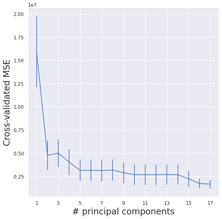
The number of components \(M\) that minimizes the MSE is 17.
pipe.named_steps['pca'].n_components = grid.best_params_['pca__n_components']
pipe.fit(X_train, y_train)
Pipeline(steps=[('scaler', StandardScaler()), ('pca', PCA(n_components=17)),
('linreg', LinearRegression())])In a Jupyter environment, please rerun this cell to show the HTML representation or trust the notebook. On GitHub, the HTML representation is unable to render, please try loading this page with nbviewer.org.
Pipeline(steps=[('scaler', StandardScaler()), ('pca', PCA(n_components=17)),
('linreg', LinearRegression())])StandardScaler()
PCA(n_components=17)
LinearRegression()
pred = pipe.predict(X_test)
pcr_MSE = np.mean((pred - y_test)**2)
pcr_MSE
642753.8976533808
This resulted in a test MSE of \(642753.90\) which is the same as fitting a linear regression with all predictors.
That’s not surpising since fitting PCR with all p predictors is equivalent to an OLS estimate.
(f)
pls = PLSRegression(scale=True)
param_grid = {'n_components':range(1, 18)}
grid = skm.GridSearchCV(pls,
param_grid,
cv=kfold,
scoring='neg_mean_squared_error')
grid.fit(X_train, y_train)
GridSearchCV(cv=KFold(n_splits=5, random_state=2, shuffle=True),
estimator=PLSRegression(),
param_grid={'n_components': range(1, 18)},
scoring='neg_mean_squared_error')In a Jupyter environment, please rerun this cell to show the HTML representation or trust the notebook. On GitHub, the HTML representation is unable to render, please try loading this page with nbviewer.org.
GridSearchCV(cv=KFold(n_splits=5, random_state=2, shuffle=True),
estimator=PLSRegression(),
param_grid={'n_components': range(1, 18)},
scoring='neg_mean_squared_error')PLSRegression(n_components=16)
PLSRegression(n_components=16)
pls_fig, ax = plt.subplots(figsize=(8,8))
n_comp = param_grid['n_components']
ax.errorbar(n_comp,
-grid.cv_results_['mean_test_score'],
grid.cv_results_['std_test_score'] / np.sqrt(K))
ax.set_ylabel('Cross-validated MSE', fontsize=20)
ax.set_xlabel('# principal components', fontsize=20)
ax.set_xticks(n_comp[::2]);
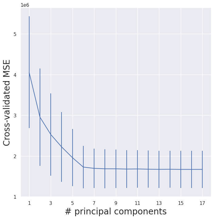
grid.best_params_
{'n_components': 16}
pls.n_components = 16
pls.fit(X_train, y_train)
PLSRegression(n_components=16)In a Jupyter environment, please rerun this cell to show the HTML representation or trust the notebook.
On GitHub, the HTML representation is unable to render, please try loading this page with nbviewer.org.
PLSRegression(n_components=16)
pred = pls.predict(X_test)
pls_MSE = np.mean((pred - y_test)**2)
pls_MSE
642728.9614907254
Cross-validation chose the value of \(M = 16\), which resulted in a test MSE of \(642728.96\). Slightly lower than the test MSE for PCR and OLS, and the lowest of all models we trained so far.
(g)
Comparing the RMSE for the models side to side we can see that PLS comes in first place followed by OLS and PCR (tied for 2nd) with a very small difference in test RMSE, Ridge in 4th place and finally Lasso in last place with a considerably higher test RMSE.
approaches = ['OLS', 'Ridge', 'Lasso', 'PCR', 'PLS']
mse_values = [ols_MSE, ridge_MSE, lasso_MSE, pcr_MSE, pls_MSE]
rmse_values = np.sqrt(mse_values)
for approach, rmse_value in zip(approaches, rmse_values):
print(f"{approach}: {rmse_value:.2f}")
OLS: 801.72
Ridge: 817.61
Lasso: 843.71
PCR: 801.72
PLS: 801.70
Plotting the results side by side.
plt.bar(approaches, rmse_values, color="skyblue", alpha=0.7)
plt.ylabel("RMSE")
plt.title("Comparison of RMSE Across The 5 Approaches")
plt.show()
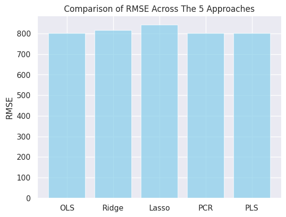
We can see that using our best model (PLS with RMSE = 801.7), our predictions, on average, deviate from the actual number of applications by about 801.7.
801.7/college['Apps'].mean()
0.26708747217842854
That error is roughly \(27\%\) of the mean value.
How good of a prediction that is depends on the context and application we plan to use this model for.
Q10.#
(a) We’ll generate \(n=1000\) observations with \(p=20\) predictors from a multivariate normal distribution with an AR(1) correlation matrix with \(\rho =0.8\).
Note: In my first attempt best_subset_selection minimized test MSE for a model of 20 predictors, which is not
allowed by the question so I increased the noise level and set more coefficients to 0, that still didn’t work so I used a multivariate normal distribution instead of a standard normal to generate the predictors.
n = 1000
p = 20
def correlation_ar1(p, rho=0.5):
"""
Returns an AR(1) correlation matrix of dimension p x p
with correlation parameter rho.
AR(1) means Corr(X_i, X_j) = rho^|i - j|.
"""
Sigma = np.zeros((p, p))
for i in range(p):
for j in range(p):
Sigma[i, j] = rho ** abs(i - j)
return Sigma
Sigma = correlation_ar1(p, rho=0.8)
sns.heatmap(Sigma);
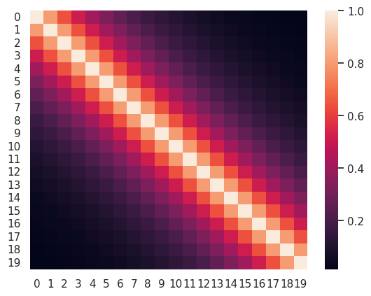
If you’re curious about the AR(1) correlation matrix that’s what it looks like, it basically means that close variables are more positively correlated with eachother.
rng = np.random.default_rng(2025)
X = rng.multivariate_normal(mean=np.zeros(p), cov=correlation_ar1(p, rho=0.8), size=n)
eps = rng.normal(0, 7, size=(n, ))
X.shape
(1000, 20)
Then we’ll create a coefficient vector \(\beta\) and generate a response vector \(Y\) according to the model:
B = np.array([2, 0, 0, 1, -2,
-1, 0, 2, 0, 0,
0, 0, 0, 0, 0,
0, 3, 0, 4, 0])
y = np.dot(X, B) + eps
y.shape
(1000,)
y[:5]
array([ -4.258917 , -7.98801827, 10.0552184 , -14.99753185,
-0.95005508])
(b)
X_train, X_test, y_train, y_test = skm.train_test_split(X, y, test_size=900, random_state=1)
X_train.shape, y_test.shape
((100, 20), (900,))
(c)
from itertools import combinations
def best_subset_selection(X_train, X_test, y_train, y_test):
p = X_train.shape[1]
best_model_for_k = {}
for k in range(p+1):
# fit the null model
if k == 0:
linreg = skl.LinearRegression().fit(np.zeros_like(X_train), y_train)
train_MSE = np.mean((linreg.predict(X_train) - y_train)**2)
pred = linreg.predict(X_test)
test_MSE = np.mean((pred - y_test)**2)
best_model_for_k[k] = ((), linreg, train_MSE, test_MSE)
continue
smallest_MSE = np.inf
# fit all p choose k combinations and pick the model with the smallest test_MSE
for subset in combinations(range(p), k):
linreg = skl.LinearRegression().fit(X_train[:,subset], y_train)
train_MSE = np.mean((linreg.predict(X_train[:,subset]) - y_train)**2)
pred = linreg.predict(X_test[:,subset])
test_MSE = np.mean((pred - y_test)**2)
if test_MSE < smallest_MSE:
best_model_for_k[k] = (subset, linreg, train_MSE, test_MSE)
return best_model_for_k
Note: This takes a few minutes to run.
best_model_for_k = best_subset_selection(X_train, X_test, y_train, y_test)
(c)
model_sizes = list(best_model_for_k.keys())
subsets = [value[0] for value in best_model_for_k.values()]
models = [value[1] for value in best_model_for_k.values()]
train_MSEs = [value[2] for value in best_model_for_k.values()]
test_MSEs = [value[3] for value in best_model_for_k.values()]
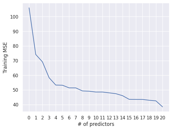
fig, ax = plt.subplots()
ax.plot(model_sizes, train_MSEs)
ax.set_xlabel('# of predictors')
ax.set_ylabel('Training MSE')
ax.set_xticks(model_sizes);
(d)
fig, ax = plt.subplots()
ax.plot(model_sizes, test_MSEs)
ax.set_xlabel('# of predictors')
ax.set_ylabel('Test MSE')
ax.set_xticks(model_sizes);
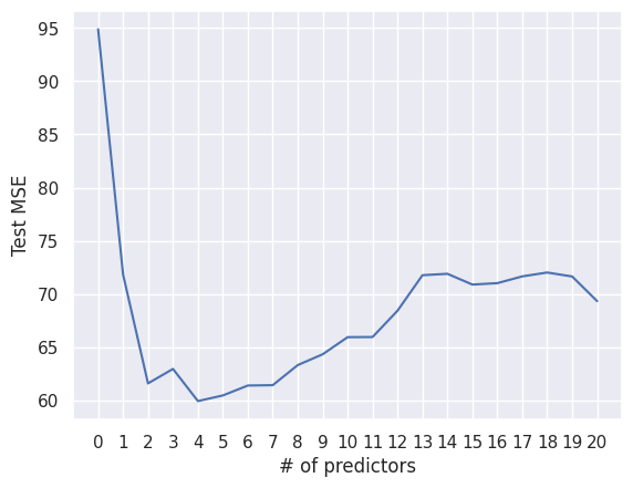
min_p = np.argmin(test_MSEs)
min_p
4
subsets[min_p], test_MSEs[min_p]
((16, 17, 18, 19), 59.94656567078981)
(e) The test set MSE takes on its minimum value for a model of size 4.
(f) Looking at the true model coefficients and the ones returned by the best subset selection:
for coef, beta in zip(models[min_p].coef_, B[list(subsets[min_p])]):
print(f"|{coef:.2f} - {beta}| = {np.abs(coef - beta):.2f}")
|3.87 - 3| = 0.87
|2.69 - 0| = 2.69
|-0.41 - 4| = 4.41
|2.13 - 0| = 2.13
Apart from the first coefficient, they’re not exaclty close to their true values, but these predictors seem to capture the correlations in the data the best.
(g) Now we’ll create a plot displaying the size of the models \(r\) on the x-axis and the euclidean distance between the true and estimated coefficient vectors (the quantity below).
# rename this properly later
euclidean_distance = {}
for r in range(1, p+1):
subset = list(subsets[r])
B_r = np.zeros(20)
for i, coef in zip(subsets[r], models[r].coef_):
B_r[i] = coef
euclidean_distance[r] = np.sqrt(np.sum((B - B_r)**2))
fig, ax = plt.subplots()
ax.plot(euclidean_distance.keys(), euclidean_distance.values())
ax.set_xlabel("# of predictors ($r$)")
ax.set_ylabel("$\\sqrt{\\sum_{j=1}^{p} (\\beta_j - \\hat\\beta_j^r)^2}$")
ax.set_xticks(list(euclidean_distance.keys()));
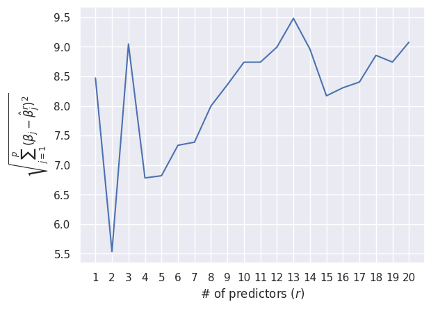
subsets[2], models[2].coef_ , B[list(subsets[2])]
((18, 19), array([3.87389325, 2.75898638]), array([4, 0]))
We can see that the plot slightly resembles the characteristic U-shape we often see for test MSE, though this one has a slight kink at \(r = 2\) where the euclidean distance is minimized, ignoring that however our best model at \(r = 4\) is a local minimum and has the 2nd lowest euclidean distance overall.
While not an indicator of model performance, euclidean distance between true and model coefficients seems like a useful guide to follow to possibly reduce the search space of subset selection methods (that is if we already have a good reference model).
Q11.#
(a)
boston = load_data('Boston')
boston.head()
| crim | zn | indus | chas | nox | rm | age | dis | rad | tax | ptratio | lstat | medv | |
|---|---|---|---|---|---|---|---|---|---|---|---|---|---|
| 0 | 0.00632 | 18.0 | 2.31 | 0 | 0.538 | 6.575 | 65.2 | 4.0900 | 1 | 296 | 15.3 | 4.98 | 24.0 |
| 1 | 0.02731 | 0.0 | 7.07 | 0 | 0.469 | 6.421 | 78.9 | 4.9671 | 2 | 242 | 17.8 | 9.14 | 21.6 |
| 2 | 0.02729 | 0.0 | 7.07 | 0 | 0.469 | 7.185 | 61.1 | 4.9671 | 2 | 242 | 17.8 | 4.03 | 34.7 |
| 3 | 0.03237 | 0.0 | 2.18 | 0 | 0.458 | 6.998 | 45.8 | 6.0622 | 3 | 222 | 18.7 | 2.94 | 33.4 |
| 4 | 0.06905 | 0.0 | 2.18 | 0 | 0.458 | 7.147 | 54.2 | 6.0622 | 3 | 222 | 18.7 | 5.33 | 36.2 |
boston.info()
<class 'pandas.core.frame.DataFrame'>
RangeIndex: 506 entries, 0 to 505
Data columns (total 13 columns):
# Column Non-Null Count Dtype
--- ------ -------------- -----
0 crim 506 non-null float64
1 zn 506 non-null float64
2 indus 506 non-null float64
3 chas 506 non-null int64
4 nox 506 non-null float64
5 rm 506 non-null float64
6 age 506 non-null float64
7 dis 506 non-null float64
8 rad 506 non-null int64
9 tax 506 non-null int64
10 ptratio 506 non-null float64
11 lstat 506 non-null float64
12 medv 506 non-null float64
dtypes: float64(10), int64(3)
memory usage: 51.5 KB
boston.describe(include='all')
| crim | zn | indus | chas | nox | rm | age | dis | rad | tax | ptratio | lstat | medv | |
|---|---|---|---|---|---|---|---|---|---|---|---|---|---|
| count | 506.000000 | 506.000000 | 506.000000 | 506.000000 | 506.000000 | 506.000000 | 506.000000 | 506.000000 | 506.000000 | 506.000000 | 506.000000 | 506.000000 | 506.000000 |
| mean | 3.613524 | 11.363636 | 11.136779 | 0.069170 | 0.554695 | 6.284634 | 68.574901 | 3.795043 | 9.549407 | 408.237154 | 18.455534 | 12.653063 | 22.532806 |
| std | 8.601545 | 23.322453 | 6.860353 | 0.253994 | 0.115878 | 0.702617 | 28.148861 | 2.105710 | 8.707259 | 168.537116 | 2.164946 | 7.141062 | 9.197104 |
| min | 0.006320 | 0.000000 | 0.460000 | 0.000000 | 0.385000 | 3.561000 | 2.900000 | 1.129600 | 1.000000 | 187.000000 | 12.600000 | 1.730000 | 5.000000 |
| 25% | 0.082045 | 0.000000 | 5.190000 | 0.000000 | 0.449000 | 5.885500 | 45.025000 | 2.100175 | 4.000000 | 279.000000 | 17.400000 | 6.950000 | 17.025000 |
| 50% | 0.256510 | 0.000000 | 9.690000 | 0.000000 | 0.538000 | 6.208500 | 77.500000 | 3.207450 | 5.000000 | 330.000000 | 19.050000 | 11.360000 | 21.200000 |
| 75% | 3.677083 | 12.500000 | 18.100000 | 0.000000 | 0.624000 | 6.623500 | 94.075000 | 5.188425 | 24.000000 | 666.000000 | 20.200000 | 16.955000 | 25.000000 |
| max | 88.976200 | 100.000000 | 27.740000 | 1.000000 | 0.871000 | 8.780000 | 100.000000 | 12.126500 | 24.000000 | 711.000000 | 22.000000 | 37.970000 | 50.000000 |
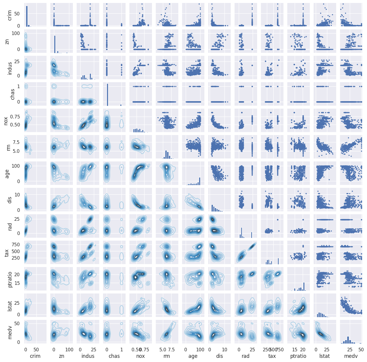
g = sns.PairGrid(boston)
g.map_upper(plt.scatter, s=3)
g.map_diag(plt.hist)
g.map_lower(sns.kdeplot, cmap="Blues_d")
g.figure.set_size_inches(12, 12)
design = MS(boston.columns.drop('crim'), intercept=False)
X = design.fit_transform(boston)
y = boston['crim']
X_train, X_test, y_train, y_test = skm.train_test_split(X, y, test_size=0.3, random_state=1)
(a)
linreg = skl.LinearRegression().fit(X_train, y_train)
pred = linreg.predict(X_test)
ols_MSE = np.mean((pred - y_test)**2)
ols_MSE
50.510476246307825
Lasso#
K = 5
kfold = skm.KFold(n_splits=K,
shuffle=True,
random_state=2)
scaler = StandardScaler()
lassoCV = skl.ElasticNetCV(l1_ratio=1,
cv=kfold)
pipeCV = Pipeline([('scaler', scaler),
('lasso', lassoCV)])
pipeCV.fit(X_train, y_train)
Pipeline(steps=[('scaler', StandardScaler()),
('lasso',
ElasticNetCV(cv=KFold(n_splits=5, random_state=2, shuffle=True),
l1_ratio=1))])In a Jupyter environment, please rerun this cell to show the HTML representation or trust the notebook. On GitHub, the HTML representation is unable to render, please try loading this page with nbviewer.org.
Pipeline(steps=[('scaler', StandardScaler()),
('lasso',
ElasticNetCV(cv=KFold(n_splits=5, random_state=2, shuffle=True),
l1_ratio=1))])StandardScaler()
ElasticNetCV(cv=KFold(n_splits=5, random_state=2, shuffle=True), l1_ratio=1)
pred = pipeCV.predict(X_test)
lasso_MSE = np.mean((pred - y_test)**2)
lasso_MSE
50.05144200256413
tuned_lasso = pipeCV.named_steps['lasso']
tuned_lasso.coef_
array([ 1.11555504, -0.45970059, -0.25950381, -1.13852783, -0.08281087,
-0. , -1.90997326, 4.91056988, -0. , -0.54943198,
1.36320495, -1.34364266])
np.sum(tuned_lasso.coef_ != 0)
10
Ridge#
K = 5
lambdas = np.linspace(0, 100, 1000)
kfold = skm.KFold(n_splits=K,
shuffle=True,
random_state=2)
scaler = StandardScaler()
ridgeCV = skl.RidgeCV(alphas=lambdas,
cv=kfold)
pipeCV = Pipeline([('scaler', scaler),
('ridge', ridgeCV)])
pipeCV.fit(X_train, y_train)
Pipeline(steps=[('scaler', StandardScaler()),
('ridge',
RidgeCV(alphas=array([ 0. , 0.1001001 , 0.2002002 , 0.3003003 ,
0.4004004 , 0.5005005 , 0.6006006 , 0.7007007 ,
0.8008008 , 0.9009009 , 1.001001 , 1.1011011 ,
1.2012012 , 1.3013013 , 1.4014014 , 1.5015015 ,
1.6016016 , 1.7017017 , 1.8018018 , 1.9019019 ,
2.002002 , 2.1021021 , 2.2022022 , 2.3023023 ,
2.4024024 , 2.5025025 , 2.6026026 , 2.7027027 ,
2.80...
97.2972973 , 97.3973974 , 97.4974975 , 97.5975976 ,
97.6976977 , 97.7977978 , 97.8978979 , 97.997998 ,
98.0980981 , 98.1981982 , 98.2982983 , 98.3983984 ,
98.4984985 , 98.5985986 , 98.6986987 , 98.7987988 ,
98.8988989 , 98.998999 , 99.0990991 , 99.1991992 ,
99.2992993 , 99.3993994 , 99.4994995 , 99.5995996 ,
99.6996997 , 99.7997998 , 99.8998999 , 100. ]),
cv=KFold(n_splits=5, random_state=2, shuffle=True)))])In a Jupyter environment, please rerun this cell to show the HTML representation or trust the notebook. On GitHub, the HTML representation is unable to render, please try loading this page with nbviewer.org.
Pipeline(steps=[('scaler', StandardScaler()),
('ridge',
RidgeCV(alphas=array([ 0. , 0.1001001 , 0.2002002 , 0.3003003 ,
0.4004004 , 0.5005005 , 0.6006006 , 0.7007007 ,
0.8008008 , 0.9009009 , 1.001001 , 1.1011011 ,
1.2012012 , 1.3013013 , 1.4014014 , 1.5015015 ,
1.6016016 , 1.7017017 , 1.8018018 , 1.9019019 ,
2.002002 , 2.1021021 , 2.2022022 , 2.3023023 ,
2.4024024 , 2.5025025 , 2.6026026 , 2.7027027 ,
2.80...
97.2972973 , 97.3973974 , 97.4974975 , 97.5975976 ,
97.6976977 , 97.7977978 , 97.8978979 , 97.997998 ,
98.0980981 , 98.1981982 , 98.2982983 , 98.3983984 ,
98.4984985 , 98.5985986 , 98.6986987 , 98.7987988 ,
98.8988989 , 98.998999 , 99.0990991 , 99.1991992 ,
99.2992993 , 99.3993994 , 99.4994995 , 99.5995996 ,
99.6996997 , 99.7997998 , 99.8998999 , 100. ]),
cv=KFold(n_splits=5, random_state=2, shuffle=True)))])StandardScaler()
RidgeCV(alphas=array([ 0. , 0.1001001 , 0.2002002 , 0.3003003 ,
0.4004004 , 0.5005005 , 0.6006006 , 0.7007007 ,
0.8008008 , 0.9009009 , 1.001001 , 1.1011011 ,
1.2012012 , 1.3013013 , 1.4014014 , 1.5015015 ,
1.6016016 , 1.7017017 , 1.8018018 , 1.9019019 ,
2.002002 , 2.1021021 , 2.2022022 , 2.3023023 ,
2.4024024 , 2.5025025 , 2.6026026 , 2.7027027 ,
2.8028028 , 2.9029029 , 3.003003 , 3.1031031 ,
3.2032032 , 3.303303...
97.2972973 , 97.3973974 , 97.4974975 , 97.5975976 ,
97.6976977 , 97.7977978 , 97.8978979 , 97.997998 ,
98.0980981 , 98.1981982 , 98.2982983 , 98.3983984 ,
98.4984985 , 98.5985986 , 98.6986987 , 98.7987988 ,
98.8988989 , 98.998999 , 99.0990991 , 99.1991992 ,
99.2992993 , 99.3993994 , 99.4994995 , 99.5995996 ,
99.6996997 , 99.7997998 , 99.8998999 , 100. ]),
cv=KFold(n_splits=5, random_state=2, shuffle=True))pipeCV.named_steps['ridge'].alpha_
42.94294294294295
pred = pipeCV.predict(X_test)
ridge_MSE = np.mean((pred - y_test)**2)
ridge_MSE
50.35785427267363
PCR#
scaler = StandardScaler()
pca = PCA(n_components=2)
linreg = skl.LinearRegression()
pipe = Pipeline([('scaler', scaler),
('pca', pca),
('linreg', linreg)])
K = 5
kfold = skm.KFold(n_splits=K,
shuffle=True,
random_state=2)
param_grid = {'pca__n_components': range(1, len(boston.columns))}
grid = skm.GridSearchCV(pipe,
param_grid,
cv=kfold,
scoring='neg_mean_squared_error')
grid.fit(X_train, y_train)
GridSearchCV(cv=KFold(n_splits=5, random_state=2, shuffle=True),
estimator=Pipeline(steps=[('scaler', StandardScaler()),
('pca', PCA(n_components=2)),
('linreg', LinearRegression())]),
param_grid={'pca__n_components': range(1, 13)},
scoring='neg_mean_squared_error')In a Jupyter environment, please rerun this cell to show the HTML representation or trust the notebook. On GitHub, the HTML representation is unable to render, please try loading this page with nbviewer.org.
GridSearchCV(cv=KFold(n_splits=5, random_state=2, shuffle=True),
estimator=Pipeline(steps=[('scaler', StandardScaler()),
('pca', PCA(n_components=2)),
('linreg', LinearRegression())]),
param_grid={'pca__n_components': range(1, 13)},
scoring='neg_mean_squared_error')Pipeline(steps=[('scaler', StandardScaler()), ('pca', PCA(n_components=12)),
('linreg', LinearRegression())])StandardScaler()
PCA(n_components=12)
LinearRegression()
grid.best_params_
{'pca__n_components': 12}
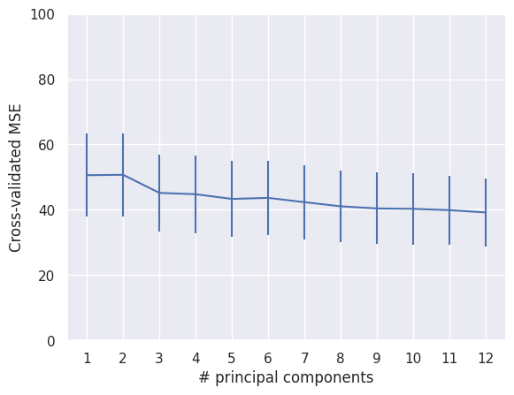
pcr_fig, ax = plt.subplots()
n_comp = param_grid['pca__n_components']
ax.errorbar(n_comp,
-grid.cv_results_['mean_test_score'],
grid.cv_results_['std_test_score'] / np.sqrt(K))
ax.set_ylabel('Cross-validated MSE')
ax.set_xlabel('# principal components')
ax.set_xticks(n_comp)
ax.set_ylim([0, 100]);
pipe.named_steps['pca'].n_components = grid.best_params_['pca__n_components']
pipe.fit(X_train, y_train)
pred = pipe.predict(X_test)
pcr_MSE = np.mean((pred - y_test)**2)
pcr_MSE
50.510476246307825
Best Subset Selection#
With a slight modification to the function above.
from itertools import combinations
def best_subset_selection(X_train, X_test, y_train, y_test):
p = X_train.shape[1]
best_model_for_k = {}
for k in range(p+1):
# fit the null model
if k == 0:
X_null = X_train.copy()
X_null.loc[:, :] = 0
linreg = skl.LinearRegression().fit(X_null, y_train)
train_MSE = np.mean((linreg.predict(X_train) - y_train)**2)
pred = linreg.predict(X_test)
test_MSE = np.mean((pred - y_test)**2)
best_model_for_k[k] = ((), linreg, train_MSE, test_MSE)
continue
smallest_MSE = np.inf
# fit all p choose k combinations and pick the model with the smallest test_MSE
for subset in combinations(range(p), k):
subset = list(subset)
linreg = skl.LinearRegression().fit(X_train.iloc[:,subset], y_train)
train_MSE = np.mean((linreg.predict(X_train.iloc[:,subset]) - y_train)**2)
pred = linreg.predict(X_test.iloc[:,subset])
test_MSE = np.mean((pred - y_test)**2)
if test_MSE < smallest_MSE:
best_model_for_k[k] = (subset, linreg, train_MSE, test_MSE)
return best_model_for_k
best_model_for_k_boston = best_subset_selection(X_train, X_test, y_train, y_test)
model_sizes = list(best_model_for_k_boston.keys())
subsets = [value[0] for value in best_model_for_k_boston.values()]
models = [value[1] for value in best_model_for_k_boston.values()]
train_MSEs = [value[2] for value in best_model_for_k_boston.values()]
test_MSEs = [value[3] for value in best_model_for_k_boston.values()]
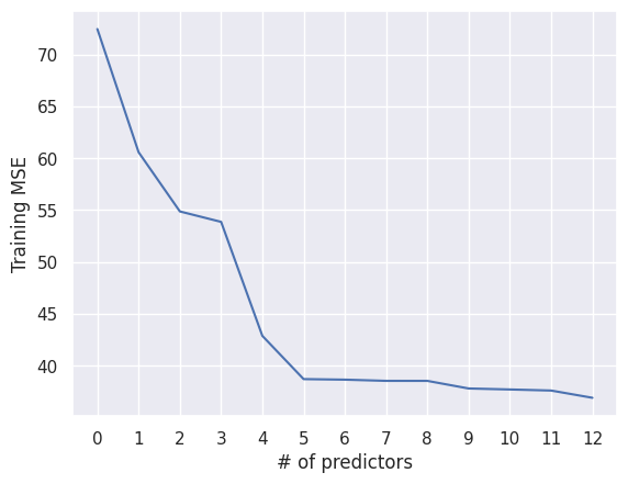
fig, ax = plt.subplots()
ax.plot(model_sizes, train_MSEs)
ax.set_xlabel('# of predictors')
ax.set_ylabel('Training MSE')
ax.set_xticks(model_sizes);
fig, ax = plt.subplots()
ax.plot(model_sizes, test_MSEs)
ax.set_xlabel('# of predictors')
ax.set_ylabel('Test MSE')
ax.set_xticks(model_sizes)
plt.scatter(model_sizes[np.argmin(test_MSEs)], np.min(test_MSEs), color='r');
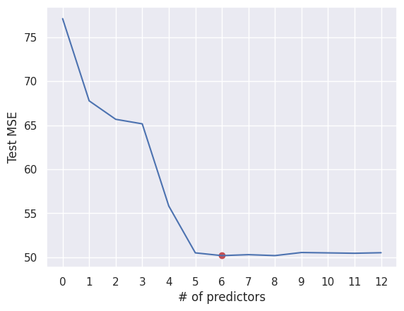
best_model_for_k_boston[np.argmin(test_MSEs)]
([6, 7, 8, 9, 10, 11],
LinearRegression(),
38.65061733583978,
50.182041497076604)
bss_MSE = best_model_for_k_boston[np.argmin(test_MSEs)][3]
bss_MSE
50.182041497076604
(b)
approaches = ['OLS', 'Ridge', 'Lasso', 'PCR', 'Best-Subset']
mse_values = [ols_MSE, ridge_MSE, lasso_MSE, pcr_MSE, bss_MSE]
rmse_values = np.sqrt(mse_values)
for approach, rmse_value in zip(approaches, rmse_values):
print(f"{approach}: {rmse_value:.2f}")
OLS: 7.11
Ridge: 7.10
Lasso: 7.07
PCR: 7.11
Best-Subset: 7.08
plt.bar(approaches, rmse_values, color="skyblue", alpha=0.7)
plt.ylabel("RMSE")
plt.title("Comparison of RMSE Across The 5 Approaches")
plt.show()
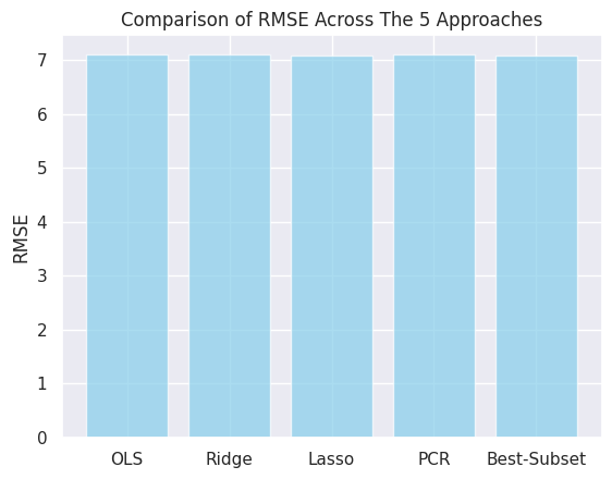
Looking at the RMSE of all 5 models we can see that the difference between them is pretty negligible. And while an RMSE of \(7\) seems pretty big when looking at the mean of \(3.6\), it’s not unreasonable when you notice how skewed the data is (ranging from \(0.00632\) to \(88.9762\) with a mean of \(3.6\) and a standard deviation of \(8.6\)). So our prediction, on average, is only off by about \(0.8\) standard deviations.
boston['crim'].mean(), boston['crim'].std(), boston['crim'].min(), boston['crim'].max()
(3.613523557312254, 8.60154510533249, 0.00632, 88.9762)
If I were to pick from the models I’d probably pick the one with the least number predictors since the difference between their RMSEs is pretty negligible.
So that’d be the model containing six predictors chosen by Best-Subset Selection.
(c) It only involved six out of twelve predictors. Because it performed just as well as or even better than the models with many or all predictors, and it’s usually better to reduce complexity whenever possible since that’d mean we can make reliable predictions with less data.