


Ch9: Support Vector Machines#
import matplotlib.pyplot as plt
import numpy as np
import seaborn as sns

sns.set_theme()

%matplotlib inline
import sklearn.linear_model as skl
import sklearn.model_selection as skm
from ISLP import load_data
from ISLP.models import ModelSpec as MS
from ISLP.svm import plot as plot_svm
from sklearn.metrics import RocCurveDisplay, accuracy_score
from sklearn.svm import SVC

roc_curve = RocCurveDisplay.from_estimator  # shorthand
Conceptual#
Q1.#
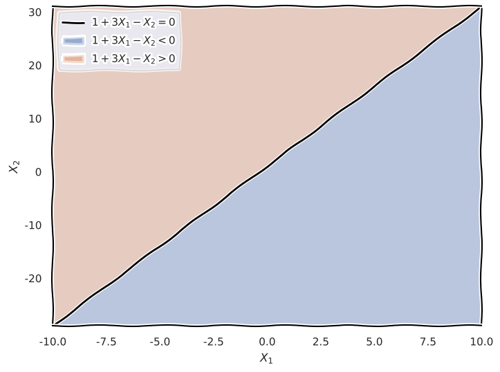
(a)
with plt.xkcd():
    plt.rcParams["font.family"] = "DejaVu Sans"  # to get rid of xkcd font warnings

    x1 = np.linspace(-10, 10, 400)
    x2 = 1 + 3 * x1

    fig, ax = plt.subplots(figsize=(8, 6))
    ax.plot(x1, x2, color="black", label=r"$ 1 + 3 X_1 - X_2 = 0 $")

    x2_min, x2_max = x2.min(), x2.max()

    ax.fill_between(x1, x2_min, x2, alpha=0.3, label=r"$ 1 + 3 X_1 - X_2 < 0 $")
    ax.fill_between(x1, x2, x2_max, alpha=0.3, label=r"$ 1 + 3 X_1 - X_2 > 0 $")

    # # remove padding so the shading fills the plot
    ax.margins(x=0, y=0)
    ax.set_xlim(x1.min(), x1.max())
    ax.set_ylim(x2_min, x2_max)

    ax.set_xlabel("$X_1$")
    ax.set_ylabel("$X_2$")
    ax.legend()
    plt.show()
(b)
with plt.xkcd():
    plt.rcParams["font.family"] = "DejaVu Sans"  # to get rid of xkcd font warnings
    x1 = np.linspace(-10, 10, 400)
    x2 = 1 - 0.5 * x1

    # fig, ax = plt.subplots()
    ax.plot(x1, x2, color="brown", label=r"$ -2 + X_1 + 2 X_2 = 0 $")

    ax.fill_between(x1, x2_min, x2, alpha=0.3, label=r"$ -2 + X_1 + 2 X_2 < 0 $")
    ax.fill_between(x1, x2, x2_max, alpha=0.3, label=r"$ -2 + X_1 + 2 X_2 > 0 $")

    ax.legend()
fig
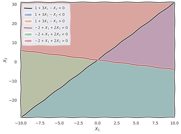
The regions are a little hard to tell apart using legend because of the overlapping colors but the question asked for both on the same plot, though it’s obvious what is referred to by each region.
Q2#
(a), (b)
with plt.xkcd():
    plt.rcParams["font.family"] = "DejaVu Sans"  # to get rid of xkcd font warnings

    def f(x, y):
        return (1 + x) ** 2 + (2 - y) ** 2 - 4

    # Create a grid of x and y values
    x1 = np.linspace(-10, 10, 400)
    x2 = np.linspace(-10, 10, 400)
    X1, X2 = np.meshgrid(x1, x2)
    Z = f(X1, X2)

    fig, ax = plt.subplots(figsize=(8, 7))

    # Plot the contour where f(x, y) = 0
    ax.contour(X1, X2, Z, levels=[0], colors="black")

    ax.contourf(X1, X2, Z, levels=[0, np.inf], colors="blue", alpha=0.5)
    ax.contourf(X1, X2, Z, levels=[-np.inf, 0], colors="red", alpha=0.5)

    # Ensure the plot isn’t distorted
    plt.gca().set_aspect("equal")
    ax.set_xlabel("$X_1$")
    ax.set_ylabel("$X_2$")
    ax.set_title("Circle: $(1 + X_1)^2 + (2 - X_2)^2 = 4$")
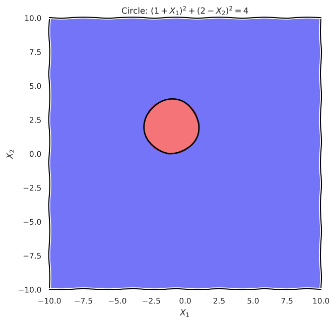
The blue region indicates the set of points for which
The red region and the black circle indicate the set of points for which
(c)
def f(x1, x2):
    return (1 + x1) ** 2 + (2 - x2) ** 2

def classify(point):
    x, y = point
    if f(x, y) > 4:
        print(f"Point ({x}, {y}) is classified as Blue.")
    elif f(x, y) < 4:
        print(f"Point ({x}, {y}) is classified as Red.")
    else:
        print(f"Point ({x}, {y}) is on the decision boundary.")
Plugging all the points into the equation for the curve, then classifiying results greater than 4 as blue and less than 4 as red:
point = (0, 0)
classify(point)
Point (0, 0) is classified as Blue.
point = (-1, 1)
classify(point)
Point (-1, 1) is classified as Red.
point = (2, 2)
classify(point)
Point (2, 2) is classified as Blue.
point = (3, 8)
classify(point)
Point (3, 8) is classified as Blue.
(d) This can be shown easily by expanding the squares:
We can see that the decision boundary here is linear in terms of \(X_1, X_1^2, X_2, X_2^2\)
Q3.#
(a)
with plt.xkcd():
    plt.rcParams["font.family"] = "DejaVu Sans"  # to get rid of xkcd font warnings

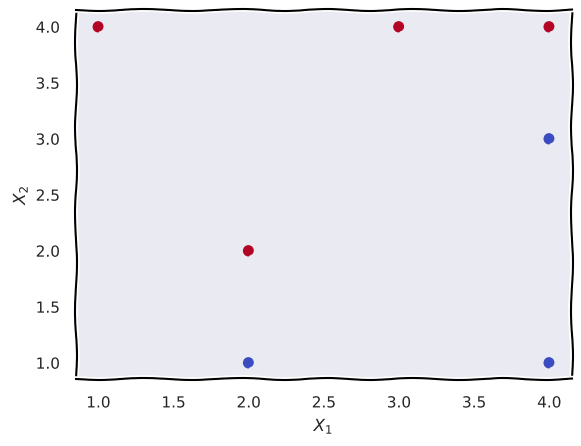
    x1 = [3, 2, 4, 1, 2, 4, 4]
    x2 = [4, 2, 4, 4, 1, 3, 1]
    y = [1, 1, 1, 1, 0, 0, 0]

    fig, ax = plt.subplots()
    ax.scatter(x1, x2, c=y, cmap=plt.cm.coolwarm)

    ax.set_xlabel("$X_1$")
    ax.set_ylabel("$X_2$")
(b)
with plt.xkcd():
    plt.rcParams["font.family"] = "DejaVu Sans"  # to get rid of xkcd font warnings

    x = np.linspace(1, 5, 100)
    osh = -0.5 + x  # optimal seperating hyperplane
    ax.plot(x, osh, color="k", label="Optimal Seperating Hyperplane")

    ax.legend()

fig
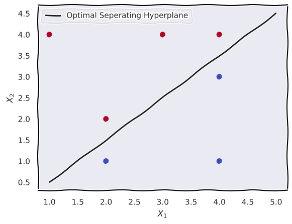
The equation for this hyperplane is:
(c) Classify as blue if:
Classify as red if:
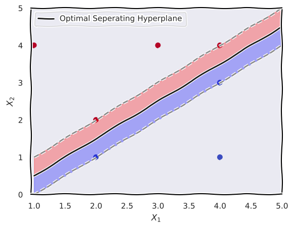
(d)
with plt.xkcd():
    plt.rcParams["font.family"] = "DejaVu Sans"  # to get rid of xkcd font warnings

    x = np.linspace(1, 5, 100)
    osh = -0.5 + x  # optimal seperating hyperplane
    margin = 0.5

    ax.plot(x, osh + margin, "k--", alpha=0.5)
    ax.plot(x, osh - margin, "k--", alpha=0.5)

    ax.fill_between(x, osh - margin, osh, color="blue", alpha=0.3)
    ax.fill_between(x, osh, osh + margin, color="red", alpha=0.3)

    ax.margins(x=0, y=0)
    ax.set_xlim([x.min() - 0.05, x.max()])

fig
(e)
with plt.xkcd():
    plt.rcParams["font.family"] = "DejaVu Sans"  # to get rid of xkcd font warnings

    support_vectors = [(2, 1), (4, 3), (2, 2), (4, 4)]
    ax.plot(*zip(*support_vectors), "*k", label="Support Vector")
    ax.legend()

fig
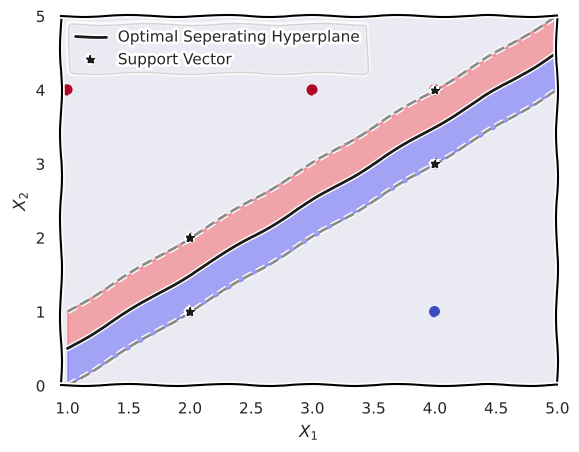
(f) The movement of the seventh observation (4, 1) would not affect the hyperplane as long as it doesn’t cross the margin, because it it’s not a support vector and our maximal margin classifier is determined using only the 4 support vectors.
(g)
with plt.xkcd():
    plt.rcParams["font.family"] = "DejaVu Sans"  # to get rid of xkcd font warnings

    x = np.linspace(1, 5, 100)
    hyperplane = 0.4 + 0.7 * x
    ax.plot(x, hyperplane, color="brown", label="hyperplane")

    ax.legend()
fig
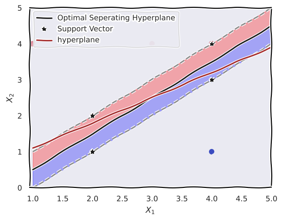
The equation for that hyperplane is:
(h)
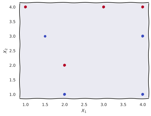
We’ll just add the observation:
with plt.xkcd():
    plt.rcParams["font.family"] = "DejaVu Sans"  # to get rid of xkcd font warnings

    x1 = [3, 2, 4, 1, 2, 4, 4]
    x2 = [4, 2, 4, 4, 1, 3, 1]
    y = [1, 1, 1, 1, 0, 0, 0]

    fig, ax = plt.subplots()
    ax.scatter(x1, x2, c=y, cmap=plt.cm.coolwarm)

    ax.set_xlabel("$X_1$")
    ax.set_ylabel("$X_2$")

    # adding a point so the points are no longer linearly seperable
    p = (1.5, 3)
    ax.scatter(p[0], p[1], c=0, cmap=plt.cm.coolwarm)
Applied#
Q4.#
rng = np.random.default_rng(10)
X = rng.standard_normal((100, 2))

X[:25] = -(X[:25] ** 2) + 4
X[75:100] = X[75:100] ** 2 - 4

y = np.array([-1] * 25 + [1] * 50 + [-1] * 25)

fig, ax = plt.subplots(figsize=(8, 8))
ax.scatter(X[:, 0], X[:, 1], c=y, cmap=plt.cm.coolwarm);
X_train, X_test, y_train, y_test = skm.train_test_split(
    X, y, test_size=0.3, random_state=1
)
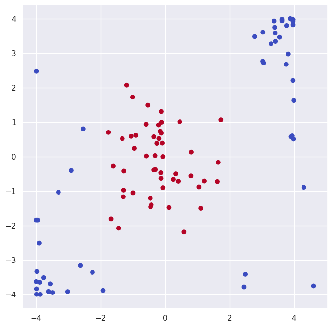
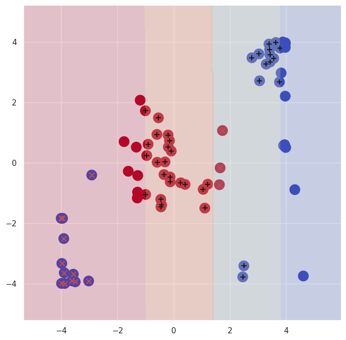
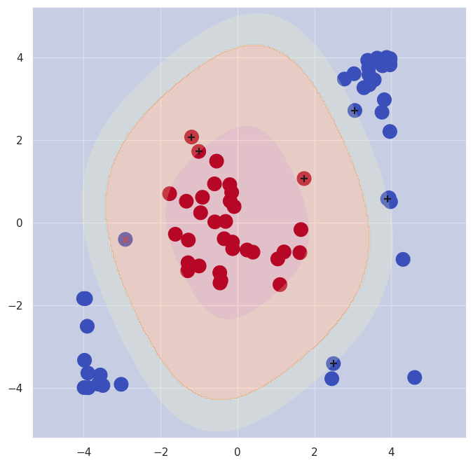
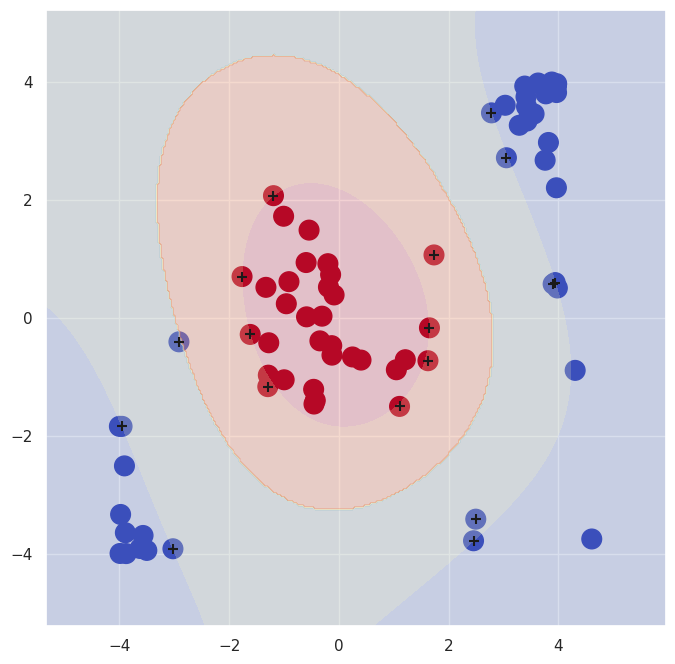
Now that we generated our data with non-linear separation, we’ll fit three SVMs with linear, polynomial and radial kernels.
svm_linear = SVC(C=10, kernel="linear")
svm_linear.fit(X_train, y_train)
fig, ax = plt.subplots(figsize=(8, 8))
plot_svm(
    X_train,
    y_train,
    svm_linear,
    ax=ax,
    decision_cmap=plt.cm.RdYlBu_r,
    scatter_cmap=plt.cm.coolwarm,
)
linear_acc = accuracy_score(y_test, svm_linear.predict(X_test))
linear_acc
0.7
svm_poly = SVC(C=1, kernel="poly", degree=4)
svm_poly.fit(X_train, y_train)
fig, ax = plt.subplots(figsize=(8, 8))
plot_svm(
    X_train,
    y_train,
    svm_poly,
    ax=ax,
    decision_cmap=plt.cm.RdYlBu_r,
    scatter_cmap=plt.cm.coolwarm,
)
poly_acc = accuracy_score(y_test, svm_poly.predict(X_test))
poly_acc
0.9666666666666667
svm_rbf = SVC(C=1, kernel="rbf")
svm_rbf.fit(X_train, y_train)
fig, ax = plt.subplots(figsize=(8, 8))
plot_svm(
    X_train,
    y_train,
    svm_rbf,
    ax=ax,
    decision_cmap=plt.cm.RdYlBu_r,
    scatter_cmap=plt.cm.coolwarm,
)
rbf_acc = accuracy_score(y_test, svm_rbf.predict(X_test))
rbf_acc
0.9666666666666667
Now we’ll print the training and test accuracy for each kernel:
Training error:
print(f"Linear: {svm_linear.score(X_train, y_train) * 100:.2f}%")
print(f"Polynomial: {svm_poly.score(X_train, y_train) * 100:.2f}%")
print(f"RBF: {svm_rbf.score(X_train, y_train) * 100:.2f}%")
Linear: 78.57%
Polynomial: 98.57%
RBF: 100.00%
Test error:
print(f"Linear: {linear_acc * 100:.2f}%")
print(f"Polynomial: {poly_acc * 100:.2f}%")
print(f"RBF: {rbf_acc * 100:.2f}%")
Linear: 70.00%
Polynomial: 96.67%
RBF: 96.67%
We can see that the SVM with the linear decision boundary performs the worst here, while the polynomial and rbf boundaries perform pretty well.
Q5.#
(a)
rng = np.random.default_rng(5)
x1 = rng.uniform(size=500) - 0.5
x2 = rng.uniform(size=500) - 0.5
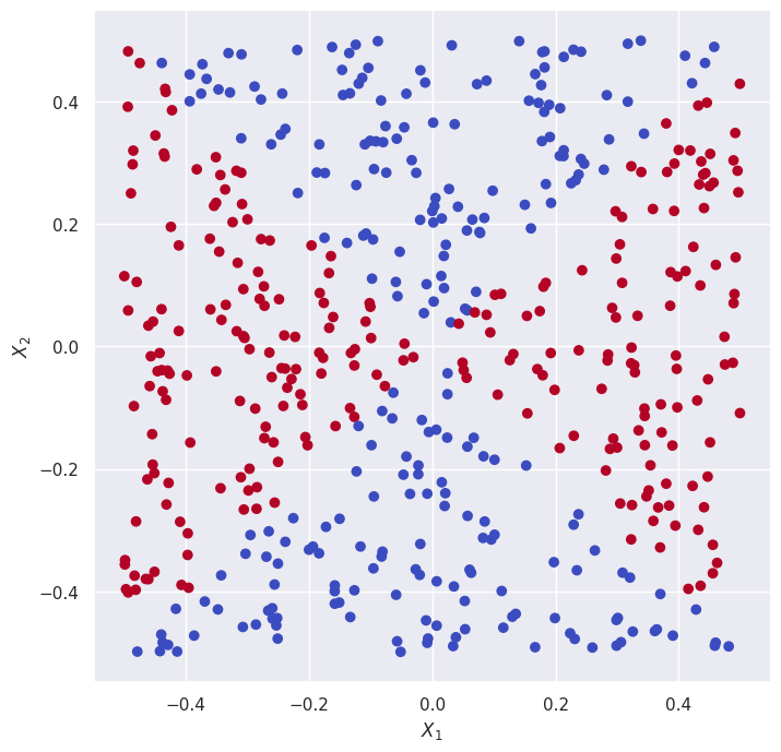
y = x1**2 - x2**2 > 0
(b)
fig, ax = plt.subplots(figsize=(8, 8))
ax.scatter(x1, x2, c=y, cmap=plt.cm.coolwarm)
ax.set_xlabel("$X_1$")
ax.set_ylabel("$X_2$");
(c)
X = np.column_stack((x1, x2))
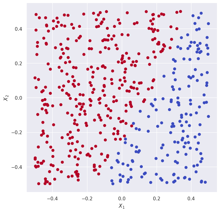
lr = skl.LogisticRegression().fit(X, y)
pred = lr.predict(X)
(d)
fig, ax = plt.subplots(figsize=(8, 8))
ax.scatter(x1, x2, c=pred, cmap=plt.cm.coolwarm)
ax.set_xlabel("$X_1$")
ax.set_ylabel("$X_2$");
(e)
X = np.column_stack((x1, np.square(x1), x2, np.square(x2)))
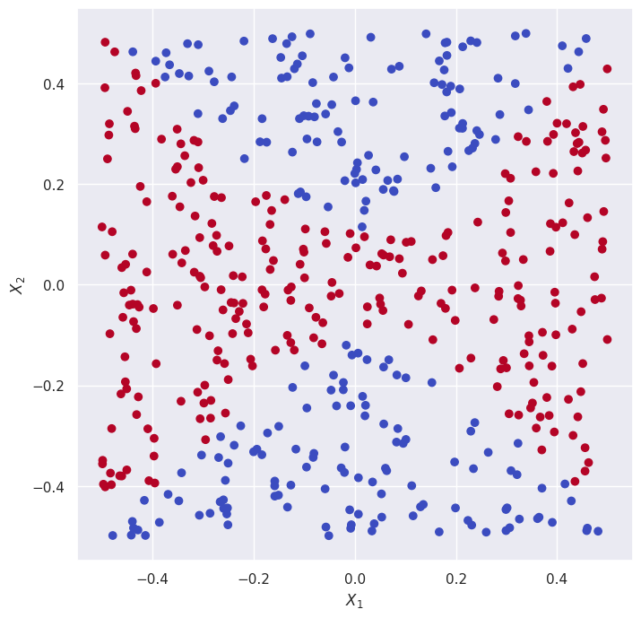
lr = skl.LogisticRegression().fit(X, y)
pred = lr.predict(X)
(f)
fig, ax = plt.subplots(figsize=(8, 8))
ax.scatter(x1, x2, c=pred, cmap=plt.cm.coolwarm)
ax.set_xlabel("$X_1$")
ax.set_ylabel("$X_2$");
(g)
X = np.column_stack((x1, x2))
svm_linear = SVC(C=10, kernel="linear").fit(X, y)
pred = svm_linear.predict(X)
fig, ax = plt.subplots(figsize=(8, 8))
ax.scatter(x1, x2, c=pred, cmap=plt.cm.coolwarm)
ax.set_xlabel("$X_1$")
ax.set_ylabel("$X_2$");
(h)
X = np.column_stack((x1, x2))
svm = SVC(C=1, kernel="rbf").fit(X, y)
pred = svm.predict(X)
fig, ax = plt.subplots(figsize=(8, 8))
ax.scatter(x1, x2, c=pred, cmap=plt.cm.coolwarm)
ax.set_xlabel("$X_1$")
ax.set_ylabel("$X_2$");
(i)
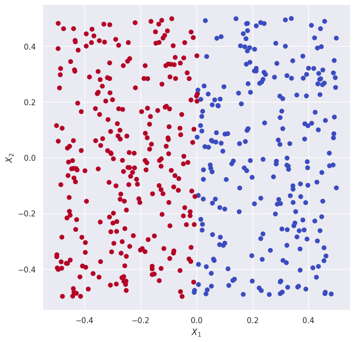
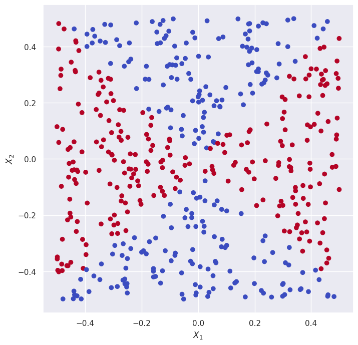
We can see that both the logistic regression fit on the original features and the linear SVM create a decision boundary that is far from the true non-linear decision boundary which is obvious considering they’re both linear methods.
The logistic regression fit using non-linear terms \(X_1, X_1^2, X_2, X_2^2\) and the SVM using the rbf kernel construct a decision boundary much closer to the true underlying decision boundary.
Q6.#
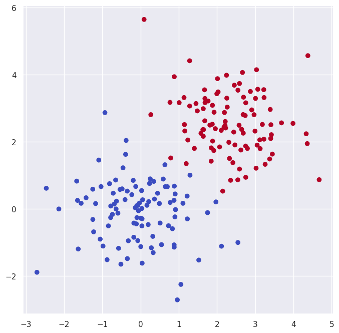
(a) Generating \(200\) observations of barely linearly separable data.
rng = np.random.default_rng(1)
X = rng.standard_normal((200, 2))
y = np.array([-1] * 100 + [1] * 100)
X[y == 1] += 2.55
fig, ax = plt.subplots(figsize=(8, 8))
ax.scatter(X[:, 0], X[:, 1], c=y, cmap=plt.cm.coolwarm);
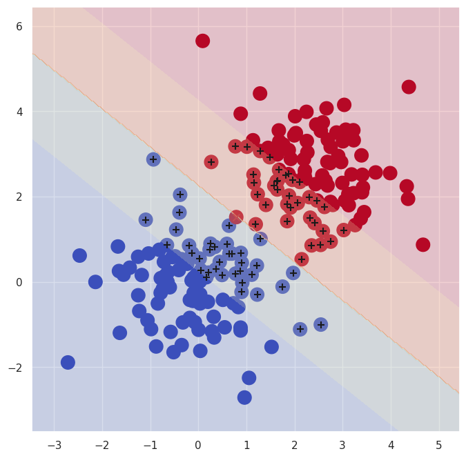
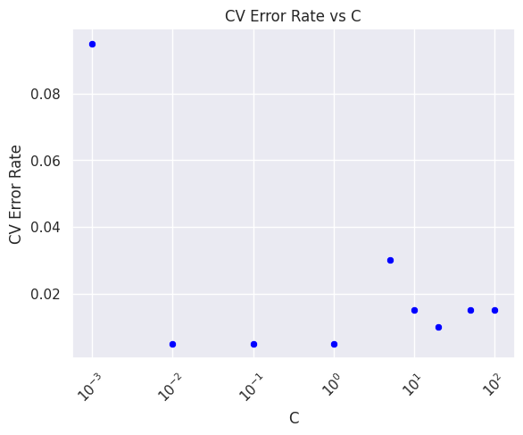
(b) Now’ll we get the cross-validation error rates for SVCs fit using the following values of C.
C_values = [0.001, 0.01, 0.1, 1, 5, 10, 20, 50, 100]
kfold = skm.KFold(n_splits=5, shuffle=True, random_state=2)

linear_svc = SVC(C=0.01, kernel="linear")

param_grid = {"C": C_values}

grid = skm.GridSearchCV(linear_svc, param_grid=param_grid, cv=kfold).fit(X, y)
grid.best_params_
{'C': 0.01}
fig, ax = plt.subplots(figsize=(8, 8))
plot_svm(
    X,
    y,
    grid.best_estimator_,
    ax=ax,
    decision_cmap=plt.cm.RdYlBu_r,
    scatter_cmap=plt.cm.coolwarm,
)
fig, ax = plt.subplots()
sns.scatterplot(
    x=C_values, y=1 - grid.cv_results_["mean_test_score"], ax=ax, color="blue"
)
ax.set_title("CV Error Rate vs C")
ax.set_xlabel("C")
ax.set_ylabel("CV Error Rate")

ax.set_xticks(C_values)
ax.set_xticklabels(C_values, rotation=45)
ax.set_xscale("log");
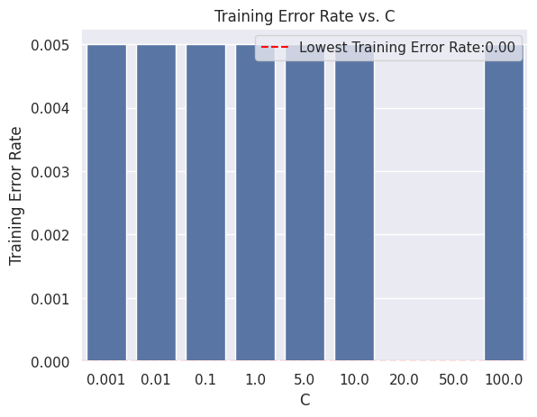
Now we’ll train a model for every value of C and save the models, training error rate, and misclassification count.
models = {}
train_err_rate = np.zeros_like(C_values)
train_mis_counts = np.zeros_like(C_values)

for idx, C in enumerate(C_values):
    linear_svc = SVC(C=C, kernel="linear")
    linear_svc.fit(X, y)

    models[C] = linear_svc
    train_err_rate[idx] = 1 - accuracy_score(y, linear_svc.predict(X))
    train_mis_counts[idx] = np.sum(linear_svc.predict(X) != y)
fig, ax = plt.subplots()
sns.barplot(x=C_values, y=train_err_rate)
ax.axhline(
    min(train_err_rate),
    color="red",
    linestyle="--",
    label=f"Lowest Training Error Rate:{min(train_err_rate):.2f}",
)
ax.legend()

ax.set_title("Training Error Rate vs. C")
ax.set_xlabel("C")
ax.set_ylabel("Training Error Rate");
fig, ax = plt.subplots()
sns.barplot(x=C_values, y=train_mis_counts)
ax.axhline(
    min(train_mis_counts),
    color="red",
    linestyle="--",
    label=f"Minimum # of Misclassifications:{min(train_mis_counts):n}",
)
ax.legend()
ax.set_title("Training # of Misclassifications vs. C")
ax.set_xlabel("C")
ax.set_ylabel("# of Misclassifications");
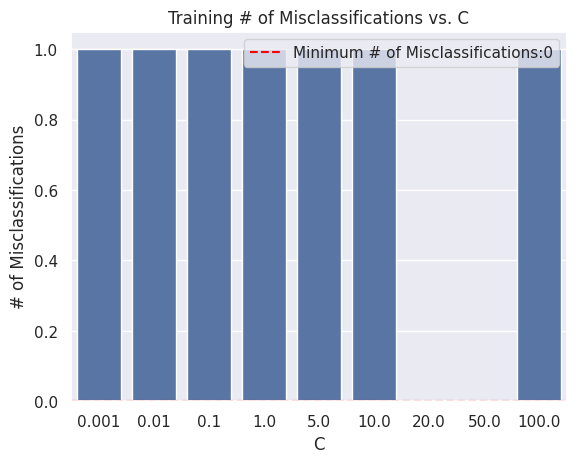
The values of C that give the lowest CV error also give the lowest misclassification error.
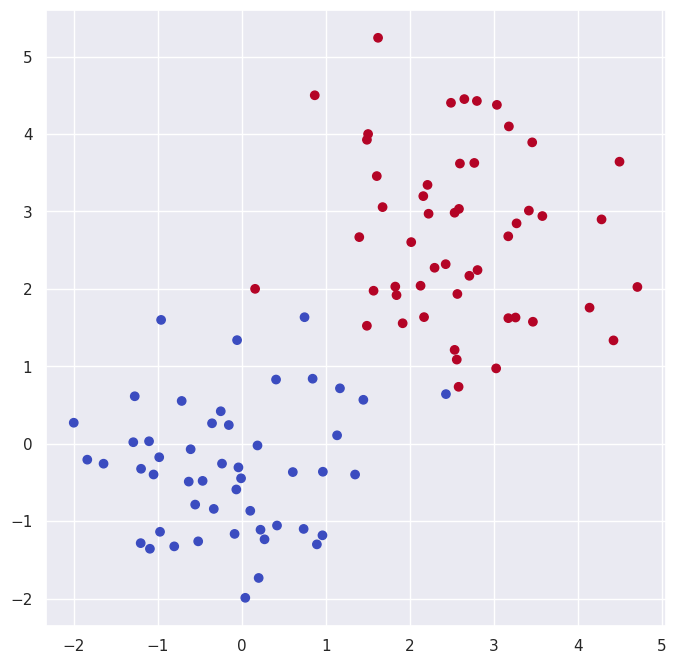
(c) Generating test data using the same method used above.
rng = np.random.default_rng(5)
X_test = rng.standard_normal((100, 2))
y_test = np.array([-1] * 50 + [1] * 50)
X_test[y_test == 1] += 2.55
fig, ax = plt.subplots(figsize=(8, 8))
ax.scatter(X_test[:, 0], X_test[:, 1], c=y_test, cmap=plt.cm.coolwarm);
Using the models we trained above to calculate the test error for each value of C.
test_err_rate = np.zeros_like(C_values)
test_mis_counts = np.zeros_like(C_values)

for idx, (C, model) in enumerate(models.items()):
    test_err_rate[idx] = 1 - accuracy_score(y_test, model.predict(X_test))
    test_mis_counts[idx] = np.sum(model.predict(X_test) != y_test)
test_err_rate, test_mis_counts
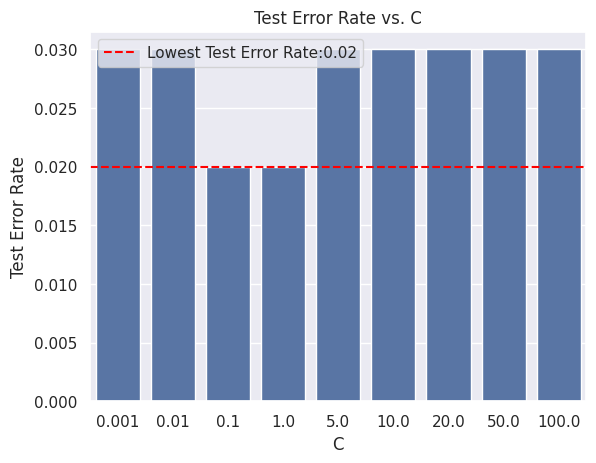
(array([0.03, 0.03, 0.02, 0.02, 0.03, 0.03, 0.03, 0.03, 0.03]),
 array([3., 3., 2., 2., 3., 3., 3., 3., 3.]))
fig, ax = plt.subplots()
sns.barplot(x=C_values, y=test_err_rate)
ax.axhline(
    min(test_err_rate),
    color="red",
    linestyle="--",
    label=f"Lowest Test Error Rate:{min(test_err_rate):.2f}",
)
ax.legend()

ax.set_title("Test Error Rate vs. C")
ax.set_xlabel("C")
ax.set_ylabel("Test Error Rate");
fig, ax = plt.subplots()
sns.barplot(x=C_values, y=test_mis_counts)
ax.axhline(
    min(test_mis_counts),
    color="red",
    linestyle="--",
    label=f"Minimum # of Misclassifications:{min(test_mis_counts):n}",
)
ax.legend()

ax.set_title("Test # of Misclassifications vs. C")
ax.set_xlabel("C")
ax.set_ylabel("# of Misclassifications");
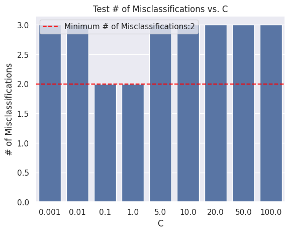
\(C = 0.1\) and \(C = 1\) lead to the fewest test errors.
They’re much smaller compared to C values that yield the fewest training errors (C = 20, C = 50). Compared to the C values that yield the lowest training error however they’re the same.
(d)
We can see that for this barely linearly seperable data even though higher values of C yielded lower training errors, lower values of C yield lower test errors.
Q7.#
auto = load_data("Auto")
auto.head()
| mpg | cylinders | displacement | horsepower | weight | acceleration | year | origin | |
|---|---|---|---|---|---|---|---|---|
| name | ||||||||
| chevrolet chevelle malibu | 18.0 | 8 | 307.0 | 130 | 3504 | 12.0 | 70 | 1 |
| buick skylark 320 | 15.0 | 8 | 350.0 | 165 | 3693 | 11.5 | 70 | 1 |
| plymouth satellite | 18.0 | 8 | 318.0 | 150 | 3436 | 11.0 | 70 | 1 |
| amc rebel sst | 16.0 | 8 | 304.0 | 150 | 3433 | 12.0 | 70 | 1 |
| ford torino | 17.0 | 8 | 302.0 | 140 | 3449 | 10.5 | 70 | 1 |
auto.info()
<class 'pandas.core.frame.DataFrame'>
Index: 392 entries, chevrolet chevelle malibu to chevy s-10
Data columns (total 8 columns):
 #   Column        Non-Null Count  Dtype
---  ------        --------------  -----
 0   mpg           392 non-null    float64
 1   cylinders     392 non-null    int64
 2   displacement  392 non-null    float64
 3   horsepower    392 non-null    int64
 4   weight        392 non-null    int64
 5   acceleration  392 non-null    float64
 6   year          392 non-null    int64
 7   origin        392 non-null    int64
dtypes: float64(3), int64(5)
memory usage: 27.6+ KB
auto.describe()
| mpg | cylinders | displacement | horsepower | weight | acceleration | year | origin | |
|---|---|---|---|---|---|---|---|---|
| count | 392.000000 | 392.000000 | 392.000000 | 392.000000 | 392.000000 | 392.000000 | 392.000000 | 392.000000 |
| mean | 23.445918 | 5.471939 | 194.411990 | 104.469388 | 2977.584184 | 15.541327 | 75.979592 | 1.576531 |
| std | 7.805007 | 1.705783 | 104.644004 | 38.491160 | 849.402560 | 2.758864 | 3.683737 | 0.805518 |
| min | 9.000000 | 3.000000 | 68.000000 | 46.000000 | 1613.000000 | 8.000000 | 70.000000 | 1.000000 |
| 25% | 17.000000 | 4.000000 | 105.000000 | 75.000000 | 2225.250000 | 13.775000 | 73.000000 | 1.000000 |
| 50% | 22.750000 | 4.000000 | 151.000000 | 93.500000 | 2803.500000 | 15.500000 | 76.000000 | 1.000000 |
| 75% | 29.000000 | 8.000000 | 275.750000 | 126.000000 | 3614.750000 | 17.025000 | 79.000000 | 2.000000 |
| max | 46.600000 | 8.000000 | 455.000000 | 230.000000 | 5140.000000 | 24.800000 | 82.000000 | 3.000000 |
(a)
auto["mpg01"] = np.where(auto["mpg"] > auto["mpg"].median(), 1, 0)
auto.head()
| mpg | cylinders | displacement | horsepower | weight | acceleration | year | origin | mpg01 | |
|---|---|---|---|---|---|---|---|---|---|
| name | |||||||||
| chevrolet chevelle malibu | 18.0 | 8 | 307.0 | 130 | 3504 | 12.0 | 70 | 1 | 0 |
| buick skylark 320 | 15.0 | 8 | 350.0 | 165 | 3693 | 11.5 | 70 | 1 | 0 |
| plymouth satellite | 18.0 | 8 | 318.0 | 150 | 3436 | 11.0 | 70 | 1 | 0 |
| amc rebel sst | 16.0 | 8 | 304.0 | 150 | 3433 | 12.0 | 70 | 1 | 0 |
| ford torino | 17.0 | 8 | 302.0 | 140 | 3449 | 10.5 | 70 | 1 | 0 |
(b)
design = MS(auto.columns.drop(["mpg", "mpg01"]), intercept=False).fit(auto)
X = design.transform(auto)
y = auto["mpg01"]
C_values = [0.001, 0.01, 0.1, 1, 5, 10, 20, 50, 100]

kfold = skm.KFold(n_splits=5, shuffle=True, random_state=1)
linear_svc = SVC(kernel="linear")
param_grid = {"C": C_values}

linear_grid = skm.GridSearchCV(linear_svc, param_grid=param_grid, cv=kfold).fit(X, y)
linear_grid.best_params_
{'C': 0.01}
errors = 1 - linear_grid.cv_results_["mean_test_score"]

fig, ax = plt.subplots()
sns.scatterplot(x=C_values, y=errors, ax=ax, color="blue")
ax.set_title("CV Error Rate vs C")
ax.set_xlabel("C")
ax.set_ylabel("CV Error Rate")

ax.set_xticks(C_values)
ax.set_xticklabels(C_values, rotation=45)
ax.set_xscale("log");
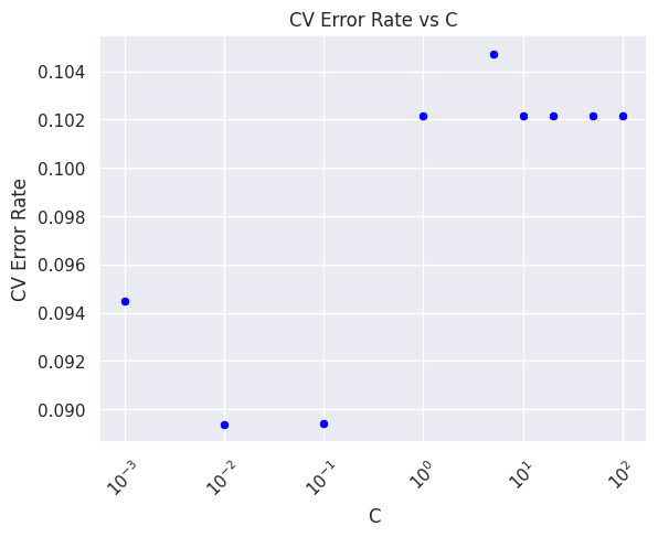
A value of \(C = 0.01\) seems to produce the lowest CV error rate.
(c)
Now we’ll repeat the process with radial and polynomial basis kernels, starting with the radial kernel.
C_values = [0.001, 0.01, 0.1, 1, 5, 10, 20, 50, 100]
gamma_values = [1e-5, 1e-4, 1e-3, 1e-2, 1e-1, 1, 10, 20, 50]

kfold = skm.KFold(n_splits=5, shuffle=True, random_state=1)
rbf_svc = SVC(kernel="rbf")
param_grid = {"C": C_values, "gamma": gamma_values}

rbf_grid = skm.GridSearchCV(rbf_svc, param_grid=param_grid, cv=kfold).fit(X, y)
rbf_grid.best_params_
{'C': 5, 'gamma': 0.0001}
rbf_grid.cv_results_["mean_test_score"]
array([0.45150925, 0.45150925, 0.45150925, 0.45150925, 0.45150925,
       0.45150925, 0.45150925, 0.45150925, 0.45150925, 0.66364817,
       0.45150925, 0.45150925, 0.45150925, 0.45150925, 0.45150925,
       0.45150925, 0.45150925, 0.45150925, 0.87241155, 0.87994158,
       0.65576112, 0.45150925, 0.45150925, 0.45150925, 0.45150925,
       0.45150925, 0.45150925, 0.869815  , 0.87234664, 0.89522882,
       0.75491723, 0.48717949, 0.46676404, 0.45150925, 0.45150925,
       0.45150925, 0.8723791 , 0.89529374, 0.88766634, 0.76514119,
       0.48974359, 0.46676404, 0.45150925, 0.45150925, 0.45150925,
       0.8723791 , 0.89013307, 0.88253814, 0.76514119, 0.48974359,
       0.46676404, 0.45150925, 0.45150925, 0.45150925, 0.8876988 ,
       0.89529374, 0.88000649, 0.76514119, 0.48974359, 0.46676404,
       0.45150925, 0.45150925, 0.45150925, 0.89023044, 0.88760143,
       0.869815  , 0.76514119, 0.48974359, 0.46676404, 0.45150925,
       0.45150925, 0.45150925, 0.88763389, 0.86471925, 0.86725089,
       0.76514119, 0.48974359, 0.46676404, 0.45150925, 0.45150925,
       0.45150925])
We’ll plot the error vs the gamma and C values on a heatmap.
rbf_errors = 1 - rbf_grid.cv_results_["mean_test_score"]
rbf_errors_2d = rbf_errors.reshape(len(gamma_values), len(C_values))

fig, ax = plt.subplots(figsize=(10, 8))
sns.heatmap(
    rbf_errors_2d,
    xticklabels=gamma_values,
    yticklabels=C_values,
    annot=True,
    fmt=".3f",
    cmap="YlGnBu_r",
    ax=ax,
)

ax.set_xlabel("$\\gamma$")
ax.set_ylabel("C")
ax.set_title("Cross-Validation Errors for SVC with RBF Kernel");
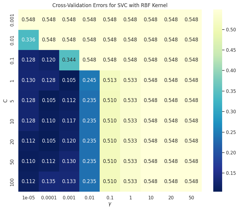
We can see that we get lower CV test errors in the dark blue regions of our heatmap, and it’s minimized for the \((C, \gamma)\) pairs \(\{(5, 0.0001), (1, 0.001), (20, 0.0001)\}\) which all result in a CV error of \(0.105\).
Using a polynomial basis kernel:
C_values = [0.001, 0.01, 0.1, 1, 5, 10, 20, 50, 100, 1000]
degrees = [2, 3, 4, 5, 6, 7, 8, 9, 10, 11]

kfold = skm.KFold(n_splits=5, shuffle=True, random_state=1)

poly_svc = SVC(kernel="poly")

param_grid = {"C": C_values, "degree": degrees}

poly_grid = skm.GridSearchCV(poly_svc, param_grid=param_grid, cv=kfold).fit(X, y)
poly_grid.best_params_
{'C': 100, 'degree': 3}
poly_errors = 1 - poly_grid.cv_results_["mean_test_score"]
poly_errors_2d = poly_errors.reshape(len(C_values), len(degrees))

fig, ax = plt.subplots(figsize=(10, 8))
sns.heatmap(
    poly_errors_2d,
    xticklabels=degrees,
    yticklabels=C_values,
    annot=True,
    fmt=".3f",
    cmap="YlGnBu_r",
    ax=ax,
)

ax.set_xlabel("Degree")
ax.set_ylabel("C")
ax.set_title("Cross-Validation Errors for SVC with Polynomial Kernel");
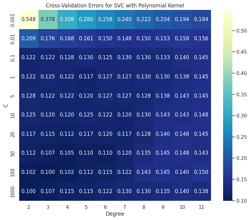
For the SVM with the polynomial kernel, we can see that the CV error is minimized at \(C=100\), degree=\(3\).
(d)
I made the plots for (b) and (c) each in its section.
Q8.#
oj = load_data("OJ")
oj.head()
| Purchase | WeekofPurchase | StoreID | PriceCH | PriceMM | DiscCH | DiscMM | SpecialCH | SpecialMM | LoyalCH | SalePriceMM | SalePriceCH | PriceDiff | Store7 | PctDiscMM | PctDiscCH | ListPriceDiff | STORE | |
|---|---|---|---|---|---|---|---|---|---|---|---|---|---|---|---|---|---|---|
| 0 | CH | 237 | 1 | 1.75 | 1.99 | 0.00 | 0.0 | 0 | 0 | 0.500000 | 1.99 | 1.75 | 0.24 | No | 0.000000 | 0.000000 | 0.24 | 1 |
| 1 | CH | 239 | 1 | 1.75 | 1.99 | 0.00 | 0.3 | 0 | 1 | 0.600000 | 1.69 | 1.75 | -0.06 | No | 0.150754 | 0.000000 | 0.24 | 1 |
| 2 | CH | 245 | 1 | 1.86 | 2.09 | 0.17 | 0.0 | 0 | 0 | 0.680000 | 2.09 | 1.69 | 0.40 | No | 0.000000 | 0.091398 | 0.23 | 1 |
| 3 | MM | 227 | 1 | 1.69 | 1.69 | 0.00 | 0.0 | 0 | 0 | 0.400000 | 1.69 | 1.69 | 0.00 | No | 0.000000 | 0.000000 | 0.00 | 1 |
| 4 | CH | 228 | 7 | 1.69 | 1.69 | 0.00 | 0.0 | 0 | 0 | 0.956535 | 1.69 | 1.69 | 0.00 | Yes | 0.000000 | 0.000000 | 0.00 | 0 |
oj.info()
<class 'pandas.core.frame.DataFrame'>
RangeIndex: 1070 entries, 0 to 1069
Data columns (total 18 columns):
 #   Column          Non-Null Count  Dtype
---  ------          --------------  -----
 0   Purchase        1070 non-null   category
 1   WeekofPurchase  1070 non-null   int64
 2   StoreID         1070 non-null   int64
 3   PriceCH         1070 non-null   float64
 4   PriceMM         1070 non-null   float64
 5   DiscCH          1070 non-null   float64
 6   DiscMM          1070 non-null   float64
 7   SpecialCH       1070 non-null   int64
 8   SpecialMM       1070 non-null   int64
 9   LoyalCH         1070 non-null   float64
 10  SalePriceMM     1070 non-null   float64
 11  SalePriceCH     1070 non-null   float64
 12  PriceDiff       1070 non-null   float64
 13  Store7          1070 non-null   category
 14  PctDiscMM       1070 non-null   float64
 15  PctDiscCH       1070 non-null   float64
 16  ListPriceDiff   1070 non-null   float64
 17  STORE           1070 non-null   int64
dtypes: category(2), float64(11), int64(5)
memory usage: 136.2 KB
oj.describe()
| WeekofPurchase | StoreID | PriceCH | PriceMM | DiscCH | DiscMM | SpecialCH | SpecialMM | LoyalCH | SalePriceMM | SalePriceCH | PriceDiff | PctDiscMM | PctDiscCH | ListPriceDiff | STORE | |
|---|---|---|---|---|---|---|---|---|---|---|---|---|---|---|---|---|
| count | 1070.000000 | 1070.000000 | 1070.000000 | 1070.000000 | 1070.000000 | 1070.000000 | 1070.000000 | 1070.000000 | 1070.000000 | 1070.000000 | 1070.000000 | 1070.000000 | 1070.000000 | 1070.000000 | 1070.000000 | 1070.000000 |
| mean | 254.381308 | 3.959813 | 1.867421 | 2.085411 | 0.051860 | 0.123364 | 0.147664 | 0.161682 | 0.565782 | 1.962047 | 1.815561 | 0.146486 | 0.059298 | 0.027314 | 0.217991 | 1.630841 |
| std | 15.558286 | 2.308984 | 0.101970 | 0.134386 | 0.117474 | 0.213834 | 0.354932 | 0.368331 | 0.307843 | 0.252697 | 0.143384 | 0.271563 | 0.101760 | 0.062232 | 0.107535 | 1.430387 |
| min | 227.000000 | 1.000000 | 1.690000 | 1.690000 | 0.000000 | 0.000000 | 0.000000 | 0.000000 | 0.000011 | 1.190000 | 1.390000 | -0.670000 | 0.000000 | 0.000000 | 0.000000 | 0.000000 |
| 25% | 240.000000 | 2.000000 | 1.790000 | 1.990000 | 0.000000 | 0.000000 | 0.000000 | 0.000000 | 0.325257 | 1.690000 | 1.750000 | 0.000000 | 0.000000 | 0.000000 | 0.140000 | 0.000000 |
| 50% | 257.000000 | 3.000000 | 1.860000 | 2.090000 | 0.000000 | 0.000000 | 0.000000 | 0.000000 | 0.600000 | 2.090000 | 1.860000 | 0.230000 | 0.000000 | 0.000000 | 0.240000 | 2.000000 |
| 75% | 268.000000 | 7.000000 | 1.990000 | 2.180000 | 0.000000 | 0.230000 | 0.000000 | 0.000000 | 0.850873 | 2.130000 | 1.890000 | 0.320000 | 0.112676 | 0.000000 | 0.300000 | 3.000000 |
| max | 278.000000 | 7.000000 | 2.090000 | 2.290000 | 0.500000 | 0.800000 | 1.000000 | 1.000000 | 0.999947 | 2.290000 | 2.090000 | 0.640000 | 0.402010 | 0.252688 | 0.440000 | 4.000000 |
oj.describe(include="category")
| Purchase | Store7 | |
|---|---|---|
| count | 1070 | 1070 |
| unique | 2 | 2 |
| top | CH | No |
| freq | 653 | 714 |
(a)
design = MS(oj.columns.drop("Purchase"), intercept=False).fit(oj)
X = design.transform(oj)
y = oj["Purchase"]
X_train, X_test, y_train, y_test = skm.train_test_split(
    X, y, train_size=800, random_state=1
)
(b)
linear_svc = SVC(C=0.01, kernel="linear").fit(X_train, y_train)
linear_svc.support_vectors_.shape
(611, 17)
There are 611 support vectors.
(c)
Training error rate:
1 - linear_svc.score(X_train, y_train)
0.31000000000000005
Test error rate:
1 - linear_svc.score(X_test, y_test)
0.3592592592592593
(d)
kfold = skm.KFold(n_splits=5, shuffle=True, random_state=3)

linear_svc = SVC(C=0.01, kernel="linear")

param_grid = {"C": np.linspace(0.01, 10, 16)}

grid = skm.GridSearchCV(linear_svc, param_grid=param_grid, cv=kfold).fit(
    X_train, y_train
)
best_linear_svc = grid.best_estimator_
best_linear_svc
SVC(C=8.668000000000001, kernel='linear')In a Jupyter environment, please rerun this cell to show the HTML representation or trust the notebook.
On GitHub, the HTML representation is unable to render, please try loading this page with nbviewer.org.
SVC(C=8.668000000000001, kernel='linear')
(e)
best_lin_train_err = 1 - best_linear_svc.score(X_train, y_train)
best_lin_test_err = 1 - best_linear_svc.score(X_test, y_test)
best_lin_train_err, best_lin_test_err
(0.16249999999999998, 0.1777777777777778)
(f)
svm_rbf = SVC(C=0.01, kernel="rbf").fit(X_train, y_train)
svm_rbf.support_vectors_.shape
(608, 17)
\(608\) support vectors.
1 - svm_rbf.score(X_train, y_train), 1 - svm_rbf.score(X_test, y_test)
(0.38, 0.4185185185185185)
svm_rbf = SVC(C=0.01, kernel="rbf")

param_grid = {"C": np.linspace(0.01, 10, 100)}

grid = skm.GridSearchCV(svm_rbf, param_grid=param_grid, cv=kfold).fit(X_train, y_train)
best_svm_rbf = grid.best_estimator_
best_svm_rbf
SVC(C=0.01)In a Jupyter environment, please rerun this cell to show the HTML representation or trust the notebook.
On GitHub, the HTML representation is unable to render, please try loading this page with nbviewer.org.
SVC(C=0.01)
best_rbf_train_err = 1 - best_svm_rbf.score(X_train, y_train)
best_rbf_test_err = 1 - best_svm_rbf.score(X_test, y_test)
best_rbf_train_err, best_rbf_test_err
(0.38, 0.4185185185185185)
(g)
svm_poly = SVC(C=0.01, kernel="poly", degree=2).fit(X_train, y_train)
svm_poly.support_vectors_.shape
(608, 17)
\(608\) support vectors.
1 - svm_poly.score(X_train, y_train), 1 - svm_poly.score(X_test, y_test)
(0.38, 0.4185185185185185)
svm_poly = SVC(C=0.01, kernel="poly", degree=2)

param_grid = {"C": np.linspace(0.01, 10, 100)}

grid = skm.GridSearchCV(svm_poly, param_grid=param_grid, cv=kfold).fit(X_train, y_train)
best_svm_poly = grid.best_estimator_
best_svm_poly
SVC(C=0.01, degree=2, kernel='poly')In a Jupyter environment, please rerun this cell to show the HTML representation or trust the notebook.
On GitHub, the HTML representation is unable to render, please try loading this page with nbviewer.org.
SVC(C=0.01, degree=2, kernel='poly')
best_poly_train_err = 1 - best_svm_poly.score(X_train, y_train)
best_poly_test_err = 1 - best_svm_poly.score(X_test, y_test)
best_poly_train_err, best_poly_test_err
(0.38, 0.4185185185185185)
(h)
We can see that the linear SVC does the best on this data out of the three methods used.
print("Training Error Rates:")
print(f"Linear: {best_lin_train_err * 100:.2f}%")
print(f"Polynomial: {best_poly_train_err * 100:.2f}%")
print(f"RBF: {best_rbf_train_err * 100:.2f}%")
Training Error Rates:
Linear: 16.25%
Polynomial: 38.00%
RBF: 38.00%
print("Test Error Rates:")
print(f"Linear: {best_lin_test_err * 100:.2f}%")
print(f"Polynomial: {best_poly_test_err * 100:.2f}%")
print(f"RBF: {best_rbf_test_err * 100:.2f}%")
Test Error Rates:
Linear: 17.78%
Polynomial: 41.85%
RBF: 41.85%