Ch2: Statistical Learning

import numpy as np
import pandas as pd
import matplotlib.pyplot as plt
import seaborn as sns

from ISLP import load_data
sns.set_theme()

%matplotlib inline

Conceptual

Q1.

Indicate whether we would generally expect the performance of a flexible statistical learning method to be better or worse than an inflexible method. Justify your answer.

a) A more flexible method would perform better in this case, as we can avoid overfitting the data because of the large sample size.

b) A less flexible model would perform better in this case, as using a more flexible model would result in overfitting the data to the small sample size.

c) A more flexible model would perform better in this case, as less flexible models tend to result in more rigid and almost linear fits which wouldn’t work in the case of our non-linear data.

d) This error term is irreducible and isn’t affected by the flexibility of our model, though we would like to find a flexibility that minimises the bias and variance of \( \hat{f}(x_0) \).

Q2.

Explain whether each scenario is a classification or regression problem, and indicate whether we are most interested in inference or prediction. Finally, provide n and p.

a) Regression, inference, n=500, p=3

b) Classification, prediction, n=20, p=13

c) Regression, prediction, n=52, p=3

Q3.

We now revisit the bias-variance decomposition.

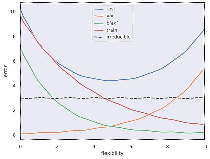
a) Provide a sketch of typical (squared) bias, variance, training error, test error, and Bayes (or irreducible) error curves, on a single plot, as we go from less flexible statistical learning methods towards more flexible approaches. The x-axis should represent the amount of flexibility in the method, and the y-axis should represent the values for each curve. There should be five curves. Make sure to label each one

with plt.xkcd():
    plt.rcParams["font.family"] = "DejaVu Sans"
    plt.figure().set_size_inches((8,6))

    x = np.linspace(0, 10, 100)

    # Rough shapes for  train, bias^2, var, test
    train = 9.5 * np.exp(-0.26 * x) + 0.1
    
    bias_sq = 7 * np.exp(-0.5 * x) + 0.1
    var     = 0.1 * np.exp(0.4* x)
    irreducible = 3
    
    test   = bias_sq + var + irreducible

    plt.xlim([0, 10])

    plt.plot(x, test,    label="test")
    plt.plot(x, var,     label="var")
    plt.plot(x, bias_sq, label="$bias^2$")
    plt.plot(x, train,   label="train")
    plt.axhline(y=irreducible, color="k", linestyle="--", label="irreducible")

    plt.xlabel("flexibility")
    plt.ylabel("error")
    plt.legend()
    plt.show()

b) Explain why each of the five curves has the shape displayed in part (a).

irreducible error curve: it has the shape of a straight horizontal line because it’s not affected by the flexibility of the model and always has the same value.

variance curve: the variance in the prediction increases as the flexibility increases.

bias^2: the squared bias decreases the more flexible the model.

test error: because it’s the sum of the irreducible error, bias^2, and variance which results in a U-shaped curve that has an asymptote at the irreducible error line.

training error: it starts off decreasing but as the flexibility increases beyond a certain point the model starts overfitting on the noise in the data which results in the curve going below the irreducible error line.

Q4.

You will now think of some real-life applications for statistical learning.

a) Classification

1. Predicting whether a certain plant is a weed or a useful plant from an image. Examples of predictors could be things like the color, shape, and other features of the plant.

2. Spam detection, predicting whether a given message is spam. Examples of predictors could be the frequency of certain words or their appearance in the message, the sender’s email/domain name.

3. Understanding what predictors affect the success of a startup company. Examples of predictors could be the market it tackles, its buisness model, its size, the amount of investment it gets during a certain period and the response is whether it succeeded or failed. (inference)

b) Regression

1. Marketing Analysis. Understanding what method of advertising increases sales the most. Predictors could be the various adverting methods and the response the number of sales. (inference)

2. Sales Forecasting. Predicting the number of sales at the end of a time period.

3. House price Forecasting. Predicting the price of a house based on its features like location, # of rooms, construction date, and other features.

c) Cluster Analysis

1. Grouping diseases together in classes based on their features.

2. Reccommendation Systems. Giving a user specific media reccs based on their media consumption history.

3. Detecting anomalies in data.

Q5.

What are the advantages and disadvantages of a very flexible (versus a less flexible) approach for regression or classification? Under what circumstances might a more flexible approach be preferred to a less flexible approach? When might a less flexible approach be preferred?

Advantages:

1. Can captures more complex and non-linear relationships better than a less flexible method.

Disadvantages:

1. More prone to overfitting than less flexible models.

A more flexible method would be preferred in situations where the sample size is sufficiently large and the underlying distribution seems to be non-linear.

A less flexible method would be preferred when the sample size is small and the underlying distribution seems to be linear.

Q6.

Describe the differences between a parametric and a non-parametric statistical learning approach. What are the advantages of a parametric approach to regression or classification (as opposed to a non-parametric approach)? What are its disadvantages?

Parametric approaches assume a specific prediction function \(f\) and try to estimate the parameters for \(f\) using the data.

Non-parametric approaches don’t make a specific assumption about \(f\) they instead try to make an estimate as close to \(f\) as possible using the data.

Advantages:

1. Less computationally intensive.

2. Easier to estimate paramters than an entire arbitrary function.

Disadvantages:

1. If the chosen model is too far from the true \(f\) then we’ll end up with poor results.

Q7.

The table below provides a training data set containing six observations, three predictors, and one qualitative response variable.

x1 = np.array([0, 2, 0, 0, -1, 1])
x2 = np.array([3, 0, 1, 1, 0, 1])
x3 = np.array([0, 0, 3, 2, 1, 1])
y = np.array([0, 0, 0, 1, 1, 0])

def euclidean_distance(obs, test_points) -> int:
    return np.sqrt(np.sum(np.abs(test_points[0] - x1[obs])**2 + np.abs(test_points[1] - x2[obs])**2 + np.abs(test_points[2] - x3[obs])**2))

test_points = [0, 0, 0]
print("(a) Euclidean distance between each observation and the test point, X1=X2=X3=0")
for i in range(6):
    print(i+1, "Green\t" if y[i] else "Red\t", euclidean_distance(i, test_points))

(a) Euclidean distance between each observation and the test point, X1=X2=X3=0
1 Red	 3.0
2 Red	 2.0
3 Red	 3.1622776601683795
4 Green	 2.23606797749979
5 Green	 1.4142135623730951
6 Red	 1.7320508075688772

(b) What is our prediction with K = 1? Why?

Green, since the closest point (5) is Green .

(c) What is our prediction with K = 3? Why?

Red, because the 3 nearest neighbors are Green, Red, Red (5, 6, 2)

(d) If the Bayes decision boundary in this problem is highly non-linear, then would we expect the best value for K to be large or small? Why

We’d expect it to be on the smaller side since smaller values of K result in more flexible fits which would work better for non-linear decision boundaries.

Applied

df = load_data('College')
df.head()

	Private	Apps	Accept	Enroll	Top10perc	Top25perc	F.Undergrad	P.Undergrad	Outstate	Room.Board	Books	Personal	PhD	Terminal	S.F.Ratio	perc.alumni	Expend	Grad.Rate
0	Yes	1660	1232	721	23	52	2885	537	7440	3300	450	2200	70	78	18.1	12	7041	60
1	Yes	2186	1924	512	16	29	2683	1227	12280	6450	750	1500	29	30	12.2	16	10527	56
2	Yes	1428	1097	336	22	50	1036	99	11250	3750	400	1165	53	66	12.9	30	8735	54
3	Yes	417	349	137	60	89	510	63	12960	5450	450	875	92	97	7.7	37	19016	59
4	Yes	193	146	55	16	44	249	869	7560	4120	800	1500	76	72	11.9	2	10922	15

df.info()

<class 'pandas.core.frame.DataFrame'>
RangeIndex: 777 entries, 0 to 776
Data columns (total 18 columns):
 #   Column       Non-Null Count  Dtype   
---  ------       --------------  -----   
 0   Private      777 non-null    category
 1   Apps         777 non-null    int64   
 2   Accept       777 non-null    int64   
 3   Enroll       777 non-null    int64   
 4   Top10perc    777 non-null    int64   
 5   Top25perc    777 non-null    int64   
 6   F.Undergrad  777 non-null    int64   
 7   P.Undergrad  777 non-null    int64   
 8   Outstate     777 non-null    int64   
 9   Room.Board   777 non-null    int64   
 10  Books        777 non-null    int64   
 11  Personal     777 non-null    int64   
 12  PhD          777 non-null    int64   
 13  Terminal     777 non-null    int64   
 14  S.F.Ratio    777 non-null    float64 
 15  perc.alumni  777 non-null    int64   
 16  Expend       777 non-null    int64   
 17  Grad.Rate    777 non-null    int64   
dtypes: category(1), float64(1), int64(16)
memory usage: 104.2 KB

df.describe(include=np.number)

	Apps	Accept	Enroll	Top10perc	Top25perc	F.Undergrad	P.Undergrad	Outstate	Room.Board	Books	Personal	PhD	Terminal	S.F.Ratio	perc.alumni	Expend	Grad.Rate
count	777.000000	777.000000	777.000000	777.000000	777.000000	777.000000	777.000000	777.000000	777.000000	777.000000	777.000000	777.000000	777.000000	777.000000	777.000000	777.000000	777.00000
mean	3001.638353	2018.804376	779.972973	27.558559	55.796654	3699.907336	855.298584	10440.669241	4357.526384	549.380952	1340.642214	72.660232	79.702703	14.089704	22.743887	9660.171171	65.46332
std	3870.201484	2451.113971	929.176190	17.640364	19.804778	4850.420531	1522.431887	4023.016484	1096.696416	165.105360	677.071454	16.328155	14.722359	3.958349	12.391801	5221.768440	17.17771
min	81.000000	72.000000	35.000000	1.000000	9.000000	139.000000	1.000000	2340.000000	1780.000000	96.000000	250.000000	8.000000	24.000000	2.500000	0.000000	3186.000000	10.00000
25%	776.000000	604.000000	242.000000	15.000000	41.000000	992.000000	95.000000	7320.000000	3597.000000	470.000000	850.000000	62.000000	71.000000	11.500000	13.000000	6751.000000	53.00000
50%	1558.000000	1110.000000	434.000000	23.000000	54.000000	1707.000000	353.000000	9990.000000	4200.000000	500.000000	1200.000000	75.000000	82.000000	13.600000	21.000000	8377.000000	65.00000
75%	3624.000000	2424.000000	902.000000	35.000000	69.000000	4005.000000	967.000000	12925.000000	5050.000000	600.000000	1700.000000	85.000000	92.000000	16.500000	31.000000	10830.000000	78.00000
max	48094.000000	26330.000000	6392.000000	96.000000	100.000000	31643.000000	21836.000000	21700.000000	8124.000000	2340.000000	6800.000000	103.000000	100.000000	39.800000	64.000000	56233.000000	118.00000

df.describe(include='category')

	Private
count	777
unique	2
top	Yes
freq	565

df.nunique()

Private          2
Apps           711
Accept         693
Enroll         581
Top10perc       82
Top25perc       89
F.Undergrad    714
P.Undergrad    566
Outstate       640
Room.Board     553
Books          122
Personal       294
PhD             78
Terminal        65
S.F.Ratio      173
perc.alumni     61
Expend         744
Grad.Rate       81
dtype: int64

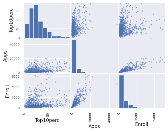
pd.plotting.scatter_matrix(df[['Top10perc', 'Apps', 'Enroll']]);

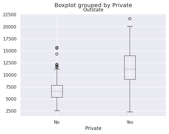
df.boxplot('Outstate', by='Private');

df['Elite'] = pd.cut(df['Top10perc']/100, 
                     [0,0.5,1],
                     labels=['No', 'Yes'])

df['Elite'].value_counts()

Elite
No     699
Yes     78
Name: count, dtype: int64

df.head()

	Private	Apps	Accept	Enroll	Top10perc	Top25perc	F.Undergrad	P.Undergrad	Outstate	Room.Board	Books	Personal	PhD	Terminal	S.F.Ratio	perc.alumni	Expend	Grad.Rate	Elite
0	Yes	1660	1232	721	23	52	2885	537	7440	3300	450	2200	70	78	18.1	12	7041	60	No
1	Yes	2186	1924	512	16	29	2683	1227	12280	6450	750	1500	29	30	12.2	16	10527	56	No
2	Yes	1428	1097	336	22	50	1036	99	11250	3750	400	1165	53	66	12.9	30	8735	54	No
3	Yes	417	349	137	60	89	510	63	12960	5450	450	875	92	97	7.7	37	19016	59	Yes
4	Yes	193	146	55	16	44	249	869	7560	4120	800	1500	76	72	11.9	2	10922	15	No

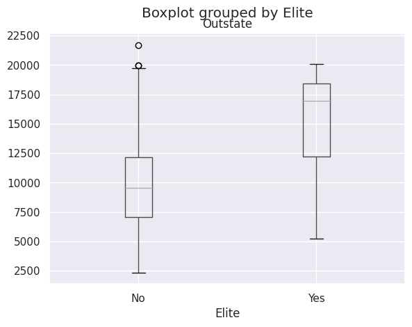
df.boxplot('Outstate', by='Elite');

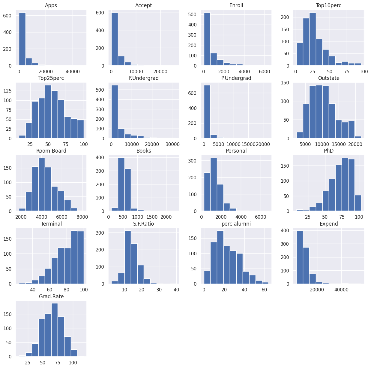
df.hist(figsize=(15,15));

Q9.

This exercise involves the Auto data set studied in the lab. Make sure that the missing values have been removed from the data

auto = load_data('Auto')

auto.head()

	mpg	cylinders	displacement	horsepower	weight	acceleration	year	origin
name
chevrolet chevelle malibu	18.0	8	307.0	130	3504	12.0	70	1
buick skylark 320	15.0	8	350.0	165	3693	11.5	70	1
plymouth satellite	18.0	8	318.0	150	3436	11.0	70	1
amc rebel sst	16.0	8	304.0	150	3433	12.0	70	1
ford torino	17.0	8	302.0	140	3449	10.5	70	1

auto.info()

<class 'pandas.core.frame.DataFrame'>
Index: 392 entries, chevrolet chevelle malibu to chevy s-10
Data columns (total 8 columns):
 #   Column        Non-Null Count  Dtype  
---  ------        --------------  -----  
 0   mpg           392 non-null    float64
 1   cylinders     392 non-null    int64  
 2   displacement  392 non-null    float64
 3   horsepower    392 non-null    int64  
 4   weight        392 non-null    int64  
 5   acceleration  392 non-null    float64
 6   year          392 non-null    int64  
 7   origin        392 non-null    int64  
dtypes: float64(3), int64(5)
memory usage: 27.6+ KB

auto.isna().sum()

mpg             0
cylinders       0
displacement    0
horsepower      0
weight          0
acceleration    0
year            0
origin          0
dtype: int64

auto.nunique()

mpg             127
cylinders         5
displacement     81
horsepower       93
weight          346
acceleration     95
year             13
origin            3
dtype: int64

(a) All are quantitative variables except the name which is used for the index.

(b) & (c)

auto.describe(include='all').loc[['mean', 'std', 'min', 'max']]

	mpg	cylinders	displacement	horsepower	weight	acceleration	year	origin
mean	23.445918	5.471939	194.411990	104.469388	2977.584184	15.541327	75.979592	1.576531
std	7.805007	1.705783	104.644004	38.491160	849.402560	2.758864	3.683737	0.805518
min	9.000000	3.000000	68.000000	46.000000	1613.000000	8.000000	70.000000	1.000000
max	46.600000	8.000000	455.000000	230.000000	5140.000000	24.800000	82.000000	3.000000

(d)

auto.iloc[10:85,].index

Index(['dodge challenger se', 'plymouth 'cuda 340', 'chevrolet monte carlo',
       'buick estate wagon (sw)', 'toyota corona mark ii', 'plymouth duster',
       'amc hornet', 'ford maverick', 'datsun pl510',
       'volkswagen 1131 deluxe sedan', 'peugeot 504', 'audi 100 ls',
       'saab 99e', 'bmw 2002', 'amc gremlin', 'ford f250', 'chevy c20',
       'dodge d200', 'hi 1200d', 'datsun pl510', 'chevrolet vega 2300',
       'toyota corona', 'amc gremlin', 'plymouth satellite custom',
       'chevrolet chevelle malibu', 'ford torino 500', 'amc matador',
       'chevrolet impala', 'pontiac catalina brougham', 'ford galaxie 500',
       'plymouth fury iii', 'dodge monaco (sw)', 'ford country squire (sw)',
       'pontiac safari (sw)', 'amc hornet sportabout (sw)',
       'chevrolet vega (sw)', 'pontiac firebird', 'ford mustang',
       'mercury capri 2000', 'opel 1900', 'peugeot 304', 'fiat 124b',
       'toyota corolla 1200', 'datsun 1200', 'volkswagen model 111',
       'plymouth cricket', 'toyota corona hardtop', 'dodge colt hardtop',
       'volkswagen type 3', 'chevrolet vega', 'ford pinto runabout',
       'chevrolet impala', 'pontiac catalina', 'plymouth fury iii',
       'ford galaxie 500', 'amc ambassador sst', 'mercury marquis',
       'buick lesabre custom', 'oldsmobile delta 88 royale',
       'chrysler newport royal', 'mazda rx2 coupe', 'amc matador (sw)',
       'chevrolet chevelle concours (sw)', 'ford gran torino (sw)',
       'plymouth satellite custom (sw)', 'volvo 145e (sw)',
       'volkswagen 411 (sw)', 'peugeot 504 (sw)', 'renault 12 (sw)',
       'ford pinto (sw)', 'datsun 510 (sw)', 'toyouta corona mark ii (sw)',
       'dodge colt (sw)', 'toyota corolla 1600 (sw)', 'buick century 350'],
      dtype='object', name='name')

auto_dropped = auto.drop(index=auto.iloc[10:85].index)

auto_dropped.info()

<class 'pandas.core.frame.DataFrame'>
Index: 282 entries, buick skylark 320 to chevy s-10
Data columns (total 8 columns):
 #   Column        Non-Null Count  Dtype  
---  ------        --------------  -----  
 0   mpg           282 non-null    float64
 1   cylinders     282 non-null    int64  
 2   displacement  282 non-null    float64
 3   horsepower    282 non-null    int64  
 4   weight        282 non-null    int64  
 5   acceleration  282 non-null    float64
 6   year          282 non-null    int64  
 7   origin        282 non-null    int64  
dtypes: float64(3), int64(5)
memory usage: 19.8+ KB

auto.describe()

	mpg	cylinders	displacement	horsepower	weight	acceleration	year	origin
count	392.000000	392.000000	392.000000	392.000000	392.000000	392.000000	392.000000	392.000000
mean	23.445918	5.471939	194.411990	104.469388	2977.584184	15.541327	75.979592	1.576531
std	7.805007	1.705783	104.644004	38.491160	849.402560	2.758864	3.683737	0.805518
min	9.000000	3.000000	68.000000	46.000000	1613.000000	8.000000	70.000000	1.000000
25%	17.000000	4.000000	105.000000	75.000000	2225.250000	13.775000	73.000000	1.000000
50%	22.750000	4.000000	151.000000	93.500000	2803.500000	15.500000	76.000000	1.000000
75%	29.000000	8.000000	275.750000	126.000000	3614.750000	17.025000	79.000000	2.000000
max	46.600000	8.000000	455.000000	230.000000	5140.000000	24.800000	82.000000	3.000000

auto_dropped.describe()

	mpg	cylinders	displacement	horsepower	weight	acceleration	year	origin
count	282.000000	282.000000	282.000000	282.000000	282.000000	282.000000	282.000000	282.000000
mean	25.006028	5.283688	180.120567	99.039007	2884.939716	15.713121	77.482270	1.631206
std	7.921384	1.637315	96.164263	34.197280	793.236373	2.601575	3.017394	0.830138
min	11.000000	3.000000	68.000000	46.000000	1755.000000	8.500000	70.000000	1.000000
25%	18.125000	4.000000	98.000000	74.250000	2188.500000	14.000000	75.000000	1.000000
50%	24.500000	4.000000	140.000000	90.000000	2715.500000	15.500000	78.000000	1.000000
75%	31.000000	6.000000	250.000000	112.000000	3435.250000	17.275000	80.000000	2.000000
max	46.600000	8.000000	455.000000	230.000000	4952.000000	24.600000	82.000000	3.000000

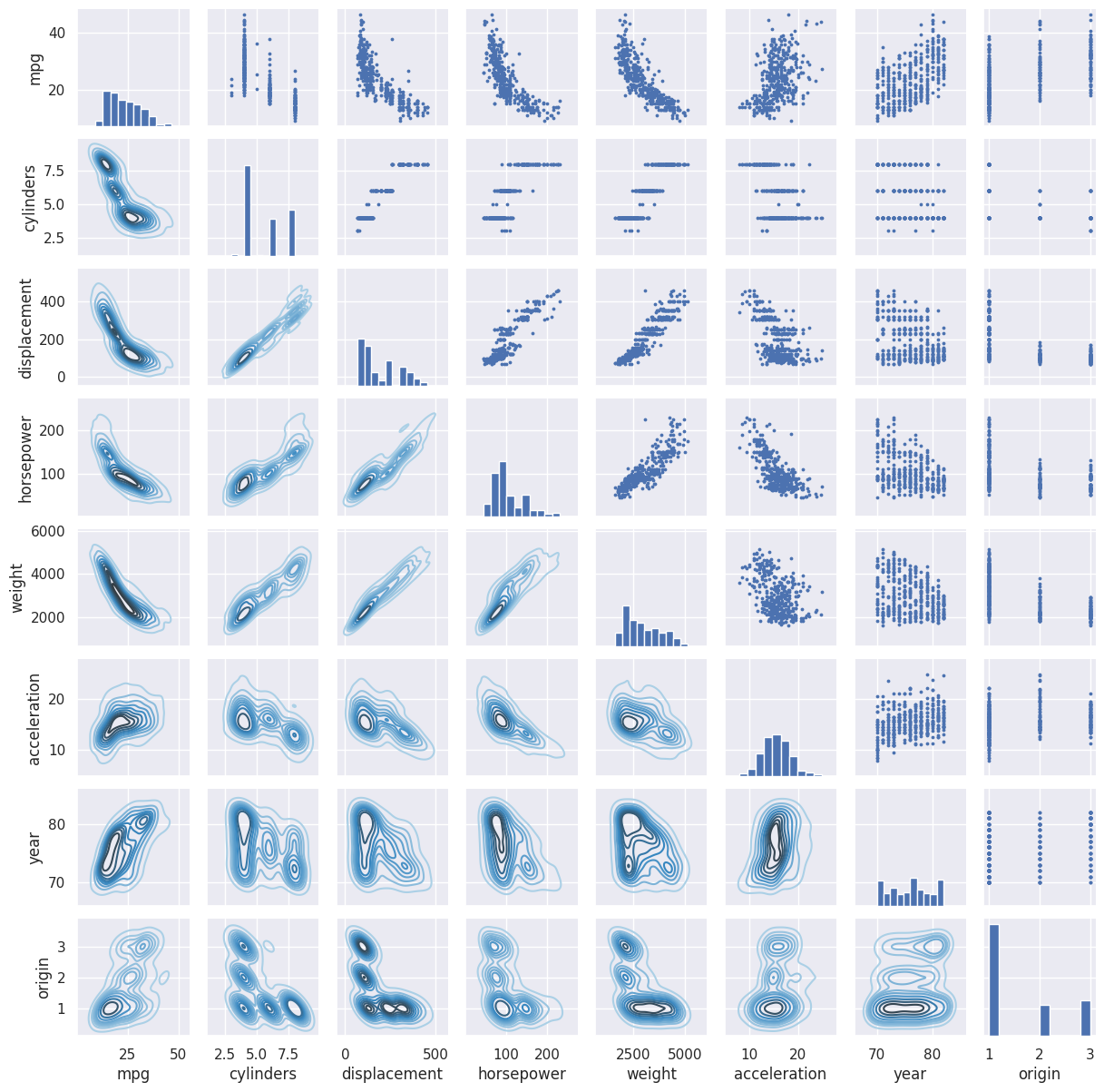
g = sns.PairGrid(auto)
g.map_upper(plt.scatter, s=3)
g.map_diag(plt.hist)
g.map_lower(sns.kdeplot, cmap="Blues_d")
g.figure.set_size_inches(12, 12)

fig, ax = plt.subplots()
fig.set_size_inches((10, 10))
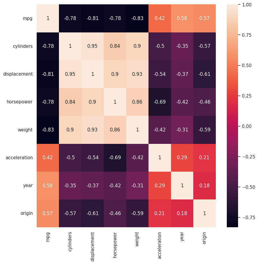
sns.heatmap(auto.corr(), annot=True);

pd.plotting.scatter_matrix(auto, figsize=(14, 14));

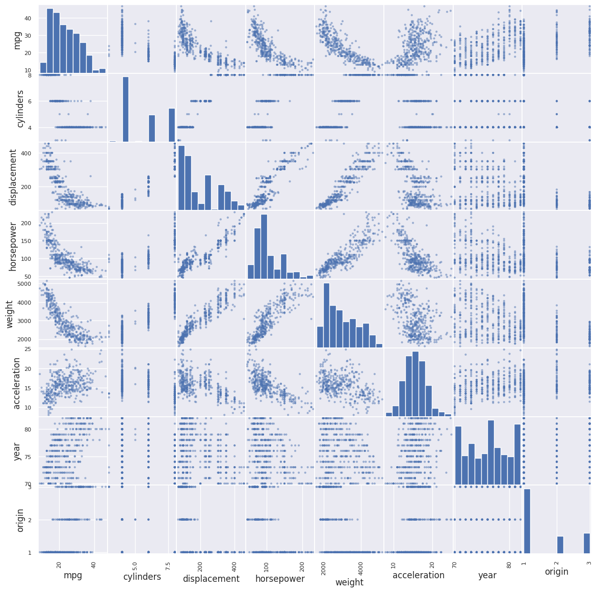
mpg seems to be negatively correlated with cylinders, weight, horsepower, and displacement, and positively correlated with acceleration, year, and origin.

(f) Yes, we can predict mpg on the basis of the other variables as there are strong correlation relationships between mpg and the other predictors.

Q10.

This exercise involves the Boston housing data set

(a)

boston = load_data('Boston')
boston.head()

	crim	zn	indus	chas	nox	rm	age	dis	rad	tax	ptratio	lstat	medv
0	0.00632	18.0	2.31	0	0.538	6.575	65.2	4.0900	1	296	15.3	4.98	24.0
1	0.02731	0.0	7.07	0	0.469	6.421	78.9	4.9671	2	242	17.8	9.14	21.6
2	0.02729	0.0	7.07	0	0.469	7.185	61.1	4.9671	2	242	17.8	4.03	34.7
3	0.03237	0.0	2.18	0	0.458	6.998	45.8	6.0622	3	222	18.7	2.94	33.4
4	0.06905	0.0	2.18	0	0.458	7.147	54.2	6.0622	3	222	18.7	5.33	36.2

boston.describe()

	crim	zn	indus	chas	nox	rm	age	dis	rad	tax	ptratio	lstat	medv
count	506.000000	506.000000	506.000000	506.000000	506.000000	506.000000	506.000000	506.000000	506.000000	506.000000	506.000000	506.000000	506.000000
mean	3.613524	11.363636	11.136779	0.069170	0.554695	6.284634	68.574901	3.795043	9.549407	408.237154	18.455534	12.653063	22.532806
std	8.601545	23.322453	6.860353	0.253994	0.115878	0.702617	28.148861	2.105710	8.707259	168.537116	2.164946	7.141062	9.197104
min	0.006320	0.000000	0.460000	0.000000	0.385000	3.561000	2.900000	1.129600	1.000000	187.000000	12.600000	1.730000	5.000000
25%	0.082045	0.000000	5.190000	0.000000	0.449000	5.885500	45.025000	2.100175	4.000000	279.000000	17.400000	6.950000	17.025000
50%	0.256510	0.000000	9.690000	0.000000	0.538000	6.208500	77.500000	3.207450	5.000000	330.000000	19.050000	11.360000	21.200000
75%	3.677083	12.500000	18.100000	0.000000	0.624000	6.623500	94.075000	5.188425	24.000000	666.000000	20.200000	16.955000	25.000000
max	88.976200	100.000000	27.740000	1.000000	0.871000	8.780000	100.000000	12.126500	24.000000	711.000000	22.000000	37.970000	50.000000

boston.info()

<class 'pandas.core.frame.DataFrame'>
RangeIndex: 506 entries, 0 to 505
Data columns (total 13 columns):
 #   Column   Non-Null Count  Dtype  
---  ------   --------------  -----  
 0   crim     506 non-null    float64
 1   zn       506 non-null    float64
 2   indus    506 non-null    float64
 3   chas     506 non-null    int64  
 4   nox      506 non-null    float64
 5   rm       506 non-null    float64
 6   age      506 non-null    float64
 7   dis      506 non-null    float64
 8   rad      506 non-null    int64  
 9   tax      506 non-null    int64  
 10  ptratio  506 non-null    float64
 11  lstat    506 non-null    float64
 12  medv     506 non-null    float64
dtypes: float64(10), int64(3)
memory usage: 51.5 KB

(b) 506 rows and 13 columns.

A data set containing housing values in 506 suburbs of Boston.

• crim: per capita crime rate by town.

• zn: proportion of residential land zoned for lots over 25,000 sq.ft.

• indus: proportion of non-retail business acres per town.

• chas: Charles River dummy variable (= 1 if tract bounds river; 0 otherwise).

• nox: nitrogen oxides concentration (parts per 10 million).

• rm: average number of rooms per dwelling.

• age: proportion of owner-occupied units built prior to 1940.

• dis: weighted mean of distances to five Boston employment centres.

• rad: index of accessibility to radial highways.

• tax: full-value property-tax rate per $10,000.

• ptratio: pupil-teacher ratio by town.

• lstat: lower status of the population (percent).

• medv: median value of owner-occupied homes in $1000s.

(c)

pd.plotting.scatter_matrix(boston, figsize=(18,18));

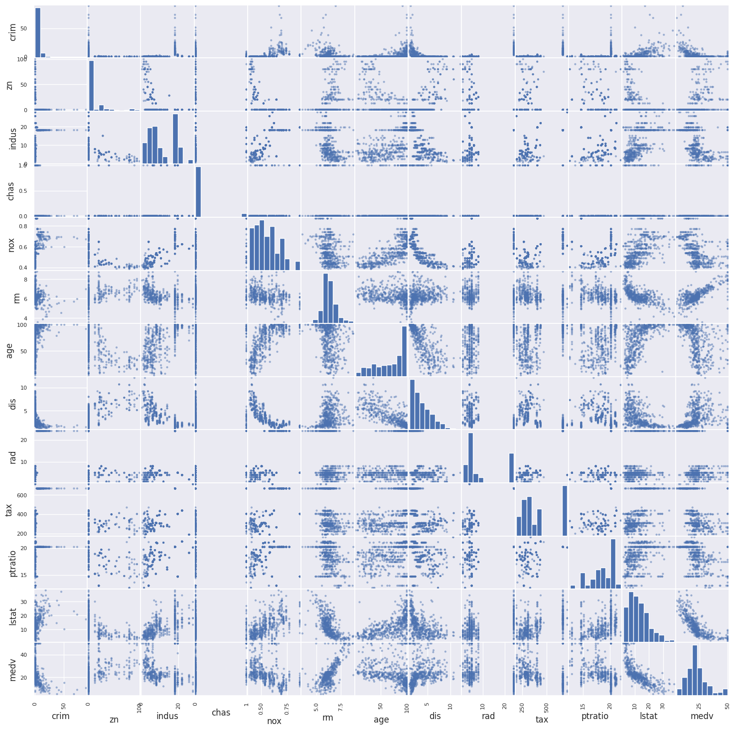
(d) medv, lstat, dis, age, nox

boston.head()

	crim	zn	indus	chas	nox	rm	age	dis	rad	tax	ptratio	lstat	medv
0	0.00632	18.0	2.31	0	0.538	6.575	65.2	4.0900	1	296	15.3	4.98	24.0
1	0.02731	0.0	7.07	0	0.469	6.421	78.9	4.9671	2	242	17.8	9.14	21.6
2	0.02729	0.0	7.07	0	0.469	7.185	61.1	4.9671	2	242	17.8	4.03	34.7
3	0.03237	0.0	2.18	0	0.458	6.998	45.8	6.0622	3	222	18.7	2.94	33.4
4	0.06905	0.0	2.18	0	0.458	7.147	54.2	6.0622	3	222	18.7	5.33	36.2

(e)

fig, axes = plt.subplots(4, 4, figsize=(16, 14))
axes = axes.flatten()

# Create boxplots using Seaborn
for i, column in enumerate(boston.columns):
    sns.boxplot(y=boston[column], ax=axes[i])
    # axes[i].set_title(column)
    
plt.tight_layout()

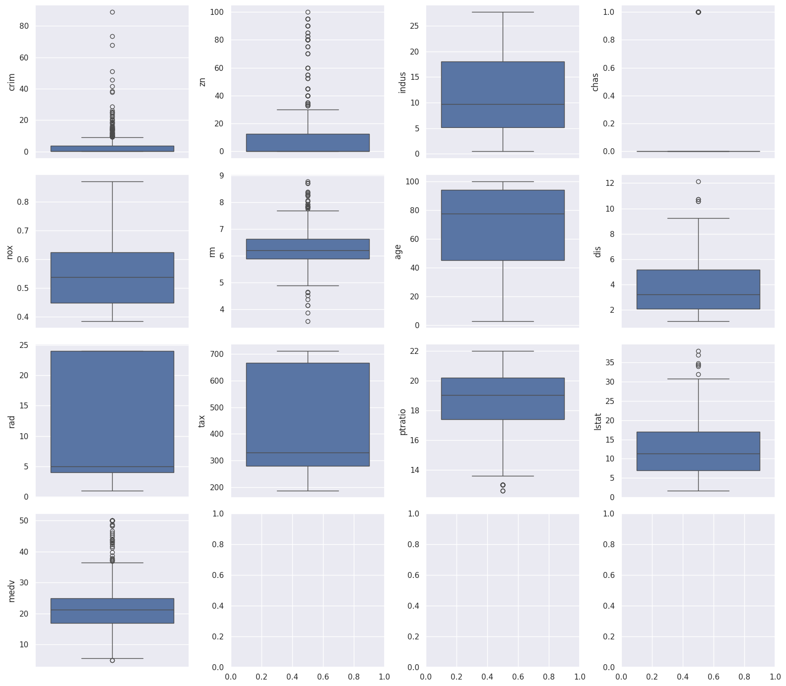
Yes there are a lot of suburbs in boston that happen to have particularly high crime rates. But tax rates and pupil-teacher ratios don’t seem to be out of the ordinary.

(f) How many of the suburbs in this data set bound the Charles river?

boston['chas'].value_counts()

chas
0    471
1     35
Name: count, dtype: int64

35 suburbs bound the Charles river.

(g) What is the median pupil-teacher ratio among the towns in this data set?

boston.median()['ptratio']

19.05

(h) Which suburb of Boston has lowest median value of owneroccupied homes? What are the values of the other predictors for that suburb, and how do those values compare to the overall ranges for those predictors? Comment on your findings.

boston.describe()

	crim	zn	indus	chas	nox	rm	age	dis	rad	tax	ptratio	lstat	medv
count	506.000000	506.000000	506.000000	506.000000	506.000000	506.000000	506.000000	506.000000	506.000000	506.000000	506.000000	506.000000	506.000000
mean	3.613524	11.363636	11.136779	0.069170	0.554695	6.284634	68.574901	3.795043	9.549407	408.237154	18.455534	12.653063	22.532806
std	8.601545	23.322453	6.860353	0.253994	0.115878	0.702617	28.148861	2.105710	8.707259	168.537116	2.164946	7.141062	9.197104
min	0.006320	0.000000	0.460000	0.000000	0.385000	3.561000	2.900000	1.129600	1.000000	187.000000	12.600000	1.730000	5.000000
25%	0.082045	0.000000	5.190000	0.000000	0.449000	5.885500	45.025000	2.100175	4.000000	279.000000	17.400000	6.950000	17.025000
50%	0.256510	0.000000	9.690000	0.000000	0.538000	6.208500	77.500000	3.207450	5.000000	330.000000	19.050000	11.360000	21.200000
75%	3.677083	12.500000	18.100000	0.000000	0.624000	6.623500	94.075000	5.188425	24.000000	666.000000	20.200000	16.955000	25.000000
max	88.976200	100.000000	27.740000	1.000000	0.871000	8.780000	100.000000	12.126500	24.000000	711.000000	22.000000	37.970000	50.000000

boston[boston['medv'] == boston['medv'].min()]

	crim	zn	indus	chas	nox	rm	age	dis	rad	tax	ptratio	lstat	medv
398	38.3518	0.0	18.1	0	0.693	5.453	100.0	1.4896	24	666	20.2	30.59	5.0
405	67.9208	0.0	18.1	0	0.693	5.683	100.0	1.4254	24	666	20.2	22.98	5.0

They’re the highest in terms of proportion of houses built prior to 1940, and have high crime rates.

len(boston[boston['rm'] > 7])

64

len(boston[boston['rm'] > 8])

13