


Ch7: Moving Beyond Linearity#
import math

import matplotlib.pyplot as plt
import numpy as np
import pandas as pd
import seaborn as sns

sns.set_theme()

%matplotlib inline
from functools import partial

import sklearn.linear_model as skl
import sklearn.model_selection as skm
import statsmodels.api as sm
from ISLP import load_data
from ISLP.models import ModelSpec as MS
from ISLP.models import Stepwise, poly, sklearn_selected, summarize
from sklearn.pipeline import Pipeline
from sklearn.preprocessing import (
    KBinsDiscretizer,
    PolynomialFeatures,
    SplineTransformer,
)
from statsmodels.stats.anova import anova_lm
from ISLP.models import bs
from ISLP.pygam import anova as anova_gam
from ISLP.pygam import plot as plot_gam
from pygam import LinearGAM
from pygam import f as f_gam
from pygam import s as s_gam
Conceptual#
Q1.#
(a) For \(x \leq \zeta \) the term \((x - \zeta)^3_+\) vanishes:
So the cubic polynomial \(f_1(x)\) that satisfies \(f(x) = f_1(x)\):
Has the following coefficients:
(b) For \(x \gt \zeta \) the term \((x - \zeta)^3_+\) equals \((x - \zeta)^3\) which can be expanded into:
Then \(f(x)\) takes the form:
For \(f_2(x) = f(x)\) to be true
The coefficients have to be:
(c) By plugging \(\zeta\) into \(f_1\) we get
Then into \(f_2\)
We can see that \(f_1(\zeta) = f_2(\zeta)\) and that \(f(x)\) is continous at \(\zeta\).
(d) We’ll start by taking the derivative of \(f_1'(x)\) and \(f_2'(x)\)
Plugging in \(\zeta\) into both functions we get:
And
We can see that
and that \(f'(x)\) is continous at \(\zeta\).
(e) We’ll differentiate again to get \(f_1''(x)\) and \(f_2''(x)\)
Plugging in \(\zeta\) into both functions we get:
And
We can see that
and that \(f''(x)\) is continous at \(\zeta\).
Q2.#
We’ll generate some values to use in our sketches below.
rng = np.random.default_rng(42)

size = 15
age = rng.normal(0, 1, size)
eps = rng.normal(0, 3, size)
y = 4*age + 0.5* age**2 * -0.6 * age**3+ eps
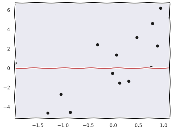
(a) For \(\lambda = \infty, m = 0\), the penalty can only be minimized when \(g^{(0)}\) is equal to \(0\), so
with plt.xkcd():
    plt.rcParams['font.family'] = 'DejaVu Sans' # to get rid of xkcd font warnings
    fig, ax = plt.subplots()
    ax.scatter(age, y, c='k')

    xs = np.linspace(-2, 2, 100)
    ax.plot(xs, np.zeros_like(xs), 'r')
    ax.set_xlim([age.min(), age.max()]);
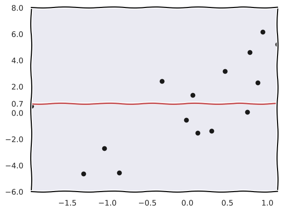
(b) For \(\lambda = \infty, m = 1\), the penalty can only be minimized when \(g^{(1)}\) the first derivative of \(g\) is equal to \(0\), so \(g\) is just a constant that minimizes the RSS term.
That constant is of course the mean of the response data points.
y.mean()
0.6994847223839016
with plt.xkcd():
    plt.rcParams['font.family'] = 'DejaVu Sans' # to get rid of xkcd font warnings

    fig, ax = plt.subplots()
    ax.scatter(age, y, c='k')

    xs = np.linspace(-2, 2, 100)
    ax.plot(xs, np.full_like(xs, y.mean()), 'r')

    yticks = np.append(ax.get_yticks(), y.mean())
    ax.set_yticks(np.sort(yticks))
    ax.set_xlim([age.min(), age.max()]);
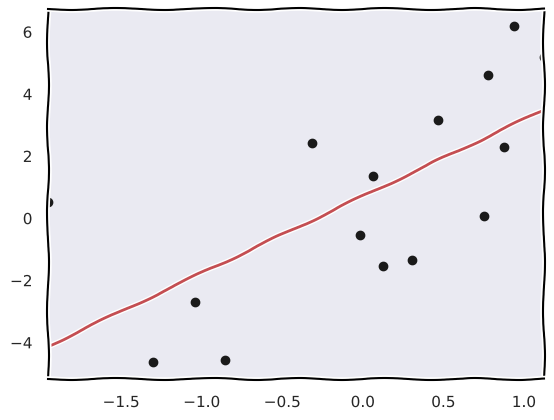
(c) For \(\lambda = \infty, m = 2\), the penalty can only be minimized when \(g^{(2)}\) the second derivative of \(g\) is equal to \(0\), so \(g\) is a linear function that minimizes the RSS term
with plt.xkcd():
    plt.rcParams['font.family'] = 'DejaVu Sans' # to get rid of xkcd font warnings

    fig, ax = plt.subplots()
    ax.scatter(age, y, c='k')

    xs = np.linspace(-2, 2, 100)

    results = sm.OLS(y, sm.add_constant(age)).fit()
    ax.plot(xs, results.predict(sm.add_constant(xs)), 'r')

    ax.set_xlim([age.min(), age.max()]);
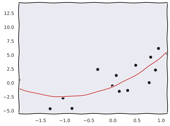
(d) For \(\lambda = \infty, m = 3\), the penalty can only be minimized when \(g^{(3)}\) the third derivative of \(g\) is equal to \(0\), so \(g\) is a quadratic function that minimizes the RSS term
with plt.xkcd():
    plt.rcParams['font.family'] = 'DejaVu Sans' # to get rid of xkcd font warnings

    fig, ax = plt.subplots()
    ax.scatter(age, y, c='k')

    xs = np.linspace(-2, 2, 100)

    X = pd.DataFrame({f'x^{i}': age**i for i in range(3)})
    results = sm.OLS(y, X).fit()
    ax.plot(xs, results.predict(pd.DataFrame({f'x^{i}': xs**i for i in range(3)})), 'r')

    ax.set_xlim([age.min(), age.max()]);
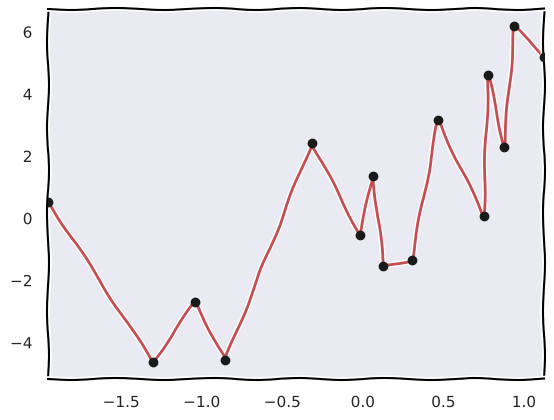
(e) For \(\lambda = 0, m = 3\), the penalty term vanishes so we only need to minimize the RSS term, which can be done using any interpolating function that connects the data points.
We’ll just connect them by straight lines since that’s the simplest way.
with plt.xkcd():
    plt.rcParams['font.family'] = 'DejaVu Sans' # to get rid of xkcd font warnings
    fig, ax = plt.subplots()
    ax.scatter(age, y, c='k', zorder=np.infty)

    sorted_indices = np.argsort(age)
    x_sorted = age[sorted_indices]
    y_sorted = y[sorted_indices]

    ax.plot(x_sorted, y_sorted, 'r')
    ax.set_xlim([age.min(), age.max()]);
Q3.#
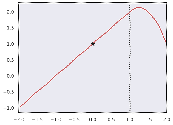
For \(X \ge 1\):
For both cases:
We can see that for \(X \ge 1\) the estimated curve is quadratic pointing down with an intercept of \(-1\).
And for \(X \lt 1\) the estimated curve is linear with an intercept and coefficient of \(1\).
def func(x):
    if x >= 1:
        return 1 + x + -2 * (x - 1)**2
    else:
        return 1 + x

age = np.linspace(-2, 2)
y = np.vectorize(func)(age)

with plt.xkcd():
    plt.rcParams['font.family'] = 'DejaVu Sans' # to get rid of xkcd font warnings
    fig, ax = plt.subplots()

    ax.plot(age, y, 'r')
    ax.axvline(1, c='k', ls=':')
    ax.set_xlim([age.min(), age.max()]);

    ax.scatter(0, 1, c='k', marker='*', s=100, zorder=np.infty)
Q4.#
Expanding the basis functions we end up with the function below:
Now we’ll create the two basis functions.
def b1(x):
    """
    b1(x) = I(0 <= x < 2) - (x - 1) I(1 <= x < 2)
    """
    term1 = ((x >= 0) & (x < 2)).astype(float)
    term2 = (x - 1) * ((x >= 1) & (x < 2)).astype(float)

    return term1 - term2

def b2(x):
    """
    b2(x) = (x - 3) I(3 <= x < 4) + I(4 <= x < 5)
    """
    term1 = (x - 3) * ((x >= 3) & (x < 4)).astype(float)
    term2 = ((x >= 4) & (x < 5)).astype(float)

    return term1 + term2
Using the coefficient estimates:
We’ll sketch this function for values between \(-2\) and \(6\).
age = np.linspace(-2, 6, 100)
y = 1 + 1 * b1(age) + 3 * b2(age)

with plt.xkcd():
    plt.rcParams['font.family'] = 'DejaVu Sans' # to get rid of xkcd font warnings
    fig, ax = plt.subplots()

    ax.plot(age, y, 'r')
    ax.set_xlim([age.min(), age.max()]);
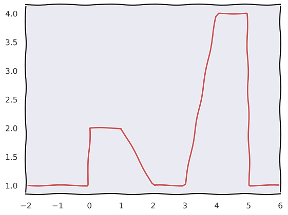
The estimated curve is split into multiple regions some are constant and some are linear according to the following function.
One thing to note is that the function is continous in the region \(0 \lt X \lt 5\), and breaks at the boundaries.
The slopes and intercepts for each region are apparent in the function above.
Q5.#
(a) \(\hat g_2\) will have a smaller training RSS since it’s a cubic model which is more flexible than the quadratic model you’d get from \(\hat g_1\).
(b) This depends on the nature of the true underlying model from which the data is generated, if it’s closer to a quadratic model \(\hat g_1\) will have the smaller RSS, if it’s cubic or more flexible than a cubic \(\hat g_2\) will have the smaller RSS.
(c) Both would have a training RSS of \(0\) since they’d have to interpolate the data points. However there are infinitely many possible functions that interpolate the training set which means the test RSS depends on how the interpolating function is chosen. If both \(\hat g_1\) and \(\hat g_2\) are chosen according to the same method then their test RSS would also be the same.
Applied#
Q6.#
wage = load_data('Wage')
wage.head()
| year | age | maritl | race | education | region | jobclass | health | health_ins | logwage | wage | |
|---|---|---|---|---|---|---|---|---|---|---|---|
| 0 | 2006 | 18 | 1. Never Married | 1. White | 1. < HS Grad | 2. Middle Atlantic | 1. Industrial | 1. <=Good | 2. No | 4.318063 | 75.043154 |
| 1 | 2004 | 24 | 1. Never Married | 1. White | 4. College Grad | 2. Middle Atlantic | 2. Information | 2. >=Very Good | 2. No | 4.255273 | 70.476020 |
| 2 | 2003 | 45 | 2. Married | 1. White | 3. Some College | 2. Middle Atlantic | 1. Industrial | 1. <=Good | 1. Yes | 4.875061 | 130.982177 |
| 3 | 2003 | 43 | 2. Married | 3. Asian | 4. College Grad | 2. Middle Atlantic | 2. Information | 2. >=Very Good | 1. Yes | 5.041393 | 154.685293 |
| 4 | 2005 | 50 | 4. Divorced | 1. White | 2. HS Grad | 2. Middle Atlantic | 2. Information | 1. <=Good | 1. Yes | 4.318063 | 75.043154 |
wage.info()
<class 'pandas.core.frame.DataFrame'>
RangeIndex: 3000 entries, 0 to 2999
Data columns (total 11 columns):
 #   Column      Non-Null Count  Dtype
---  ------      --------------  -----
 0   year        3000 non-null   int64
 1   age         3000 non-null   int64
 2   maritl      3000 non-null   category
 3   race        3000 non-null   category
 4   education   3000 non-null   category
 5   region      3000 non-null   category
 6   jobclass    3000 non-null   category
 7   health      3000 non-null   category
 8   health_ins  3000 non-null   category
 9   logwage     3000 non-null   float64
 10  wage        3000 non-null   float64
dtypes: category(7), float64(2), int64(2)
memory usage: 115.5 KB
wage.describe(include='number')
| year | age | logwage | wage | |
|---|---|---|---|---|
| count | 3000.000000 | 3000.000000 | 3000.000000 | 3000.000000 |
| mean | 2005.791000 | 42.414667 | 4.653905 | 111.703608 |
| std | 2.026167 | 11.542406 | 0.351753 | 41.728595 |
| min | 2003.000000 | 18.000000 | 3.000000 | 20.085537 |
| 25% | 2004.000000 | 33.750000 | 4.447158 | 85.383940 |
| 50% | 2006.000000 | 42.000000 | 4.653213 | 104.921507 |
| 75% | 2008.000000 | 51.000000 | 4.857332 | 128.680488 |
| max | 2009.000000 | 80.000000 | 5.763128 | 318.342430 |
wage.describe(include='category')
| maritl | race | education | region | jobclass | health | health_ins | |
|---|---|---|---|---|---|---|---|
| count | 3000 | 3000 | 3000 | 3000 | 3000 | 3000 | 3000 |
| unique | 5 | 4 | 5 | 1 | 2 | 2 | 2 |
| top | 2. Married | 1. White | 2. HS Grad | 2. Middle Atlantic | 1. Industrial | 2. >=Very Good | 1. Yes |
| freq | 2074 | 2480 | 971 | 3000 | 1544 | 2142 | 2083 |
age = wage['age']
y = wage['wage']

kfold = skm.KFold(5, shuffle=True, random_state=1)

params = {"poly__degree": np.arange(1, 20)}

polyPipe = Pipeline([("poly", PolynomialFeatures()),
                     ("linreg", skl.LinearRegression())])

cv_results = skm.GridSearchCV(polyPipe, param_grid=params, cv=kfold).fit(np.reshape(age, (-1, 1)), y)
cv_results
GridSearchCV(cv=KFold(n_splits=5, random_state=1, shuffle=True),
             estimator=Pipeline(steps=[('poly', PolynomialFeatures()),
                                       ('linreg', LinearRegression())]),
             param_grid={'poly__degree': array([ 1,  2,  3,  4,  5,  6,  7,  8,  9, 10, 11, 12, 13, 14, 15, 16, 17,
       18, 19])})
In a Jupyter environment, please rerun this cell to show the HTML representation or trust the notebook. On GitHub, the HTML representation is unable to render, please try loading this page with nbviewer.org.
GridSearchCV(cv=KFold(n_splits=5, random_state=1, shuffle=True),
             estimator=Pipeline(steps=[('poly', PolynomialFeatures()),
                                       ('linreg', LinearRegression())]),
             param_grid={'poly__degree': array([ 1,  2,  3,  4,  5,  6,  7,  8,  9, 10, 11, 12, 13, 14, 15, 16, 17,
18, 19])})Pipeline(steps=[('poly', PolynomialFeatures(degree=7)),
('linreg', LinearRegression())])PolynomialFeatures(degree=7)
LinearRegression()
best_degree = cv_results.best_params_['poly__degree']
best_degree
7
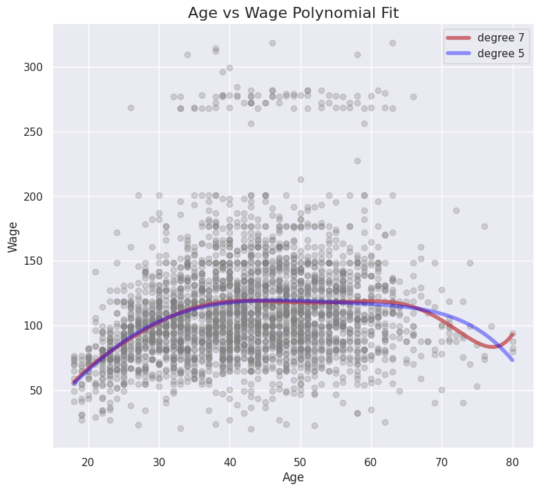
The optimal degree for the polynomial chosen by cross-validation is \(7\).
models = [MS([poly('age', degree=d)])
for d in range(1, best_degree+1)]
Xs = [model.fit_transform(wage) for model in models]
anova_lm(*[sm.OLS(y, X_).fit()
for X_ in Xs])
| df_resid | ssr | df_diff | ss_diff | F | Pr(>F) | |
|---|---|---|---|---|---|---|
| 0 | 2998.0 | 5.022216e+06 | 0.0 | NaN | NaN | NaN |
| 1 | 2997.0 | 4.793430e+06 | 1.0 | 228786.010128 | 143.692606 | 2.253516e-32 |
| 2 | 2996.0 | 4.777674e+06 | 1.0 | 15755.693664 | 9.895608 | 1.672982e-03 |
| 3 | 2995.0 | 4.771604e+06 | 1.0 | 6070.152124 | 3.812453 | 5.096592e-02 |
| 4 | 2994.0 | 4.770322e+06 | 1.0 | 1282.563017 | 0.805534 | 3.695162e-01 |
| 5 | 2993.0 | 4.766389e+06 | 1.0 | 3932.257665 | 2.469715 | 1.161646e-01 |
| 6 | 2992.0 | 4.763834e+06 | 1.0 | 2555.281281 | 1.604884 | 2.053110e-01 |
Which is different from the best degree we’d pick by following the ANOVA results \((5)\).
bestPoly = cv_results.best_estimator_
bestPoly
Pipeline(steps=[('poly', PolynomialFeatures(degree=7)),
('linreg', LinearRegression())])In a Jupyter environment, please rerun this cell to show the HTML representation or trust the notebook. On GitHub, the HTML representation is unable to render, please try loading this page with nbviewer.org.
Pipeline(steps=[('poly', PolynomialFeatures(degree=7)),
('linreg', LinearRegression())])PolynomialFeatures(degree=7)
LinearRegression()
fig, ax = plt.subplots(figsize=(9,8))
ax.scatter(age, y, alpha=0.3, c='gray')

# plotting the 7 degree polynomial
xs = np.linspace(age.min(), age.max(), 1000).reshape((-1, 1))
ax.plot(xs, bestPoly.predict(xs), lw=4, c='r', alpha=0.8, label='degree 7')

# fitting and plotting the 5 degree polynomial
polyPipe5 = Pipeline([("poly", PolynomialFeatures(5)),
                     ("linreg", skl.LinearRegression())]).fit(np.reshape(age,(-1,1)), y)

ax.plot(xs, polyPipe5.predict(xs), lw=4, c='blue', alpha=0.4, label='degree 5')


ax.set_title('Age vs Wage Polynomial Fit', fontsize=16)
ax.set_xlabel('Age')
ax.set_ylabel('Wage')
ax.legend();
(b)
pipeCut = Pipeline([
    ('discretizer', KBinsDiscretizer(encode='onehot-dense', strategy='uniform')),
    ('linreg', skl.LinearRegression())
])

param_grid = {
    'discretizer__n_bins': np.arange(2, 21)  # trying from 2 to 20 bins (1 to 19 cuts)
}

cv_results = skm.GridSearchCV(pipeCut, param_grid, cv=kfold).fit(np.reshape(age, (-1, 1)), y)
cv_results.best_params_
{'discretizer__n_bins': 16}
best_estimator = cv_results.best_estimator_
best_estimator
Pipeline(steps=[('discretizer',
                 KBinsDiscretizer(encode='onehot-dense', n_bins=16,
                                  strategy='uniform')),
                ('linreg', LinearRegression())])
In a Jupyter environment, please rerun this cell to show the HTML representation or trust the notebook. On GitHub, the HTML representation is unable to render, please try loading this page with nbviewer.org.
Pipeline(steps=[('discretizer',
                 KBinsDiscretizer(encode='onehot-dense', n_bins=16,
                                  strategy='uniform')),
('linreg', LinearRegression())])KBinsDiscretizer(encode='onehot-dense', n_bins=16, strategy='uniform')
LinearRegression()
best_cut = cv_results.best_params_['discretizer__n_bins']
best_cut
16
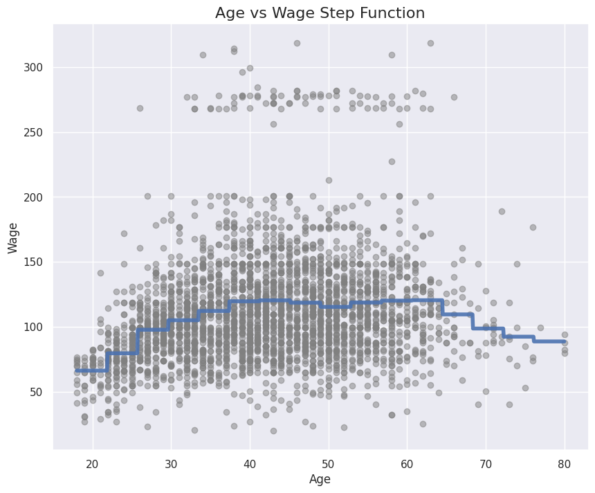
The optimal number of bins chosen by cross-validation is \(16\) (\(15\) cuts).
fig, ax = plt.subplots(figsize=(10,8))
ax.scatter(age, y, facecolor='gray', alpha=0.5)

new_age = np.linspace(age.min(), age.max(), 1000).reshape(-1, 1)
ax.plot(new_age, best_estimator.predict(new_age), 'b-', linewidth=4, alpha=0.9)

ax.set_title('Age vs Wage Step Function', fontsize=16)
ax.set_xlabel('Age')
ax.set_ylabel('Wage');
Q7.#
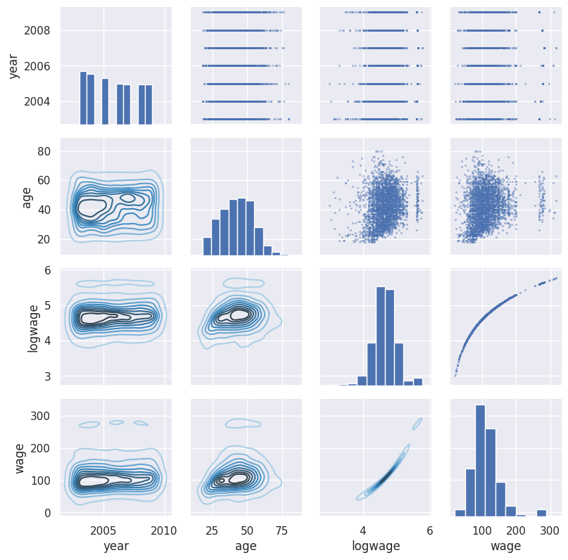
We’ll create some plots of the quantitative variables first to understand them better.
g = sns.PairGrid(wage)
g.map_upper(plt.scatter, s=3, linewidths=0.4, alpha=0.4)
g.map_diag(plt.hist)
g.map_lower(sns.kdeplot, cmap="Blues_d")
g.figure.set_size_inches(8, 8)
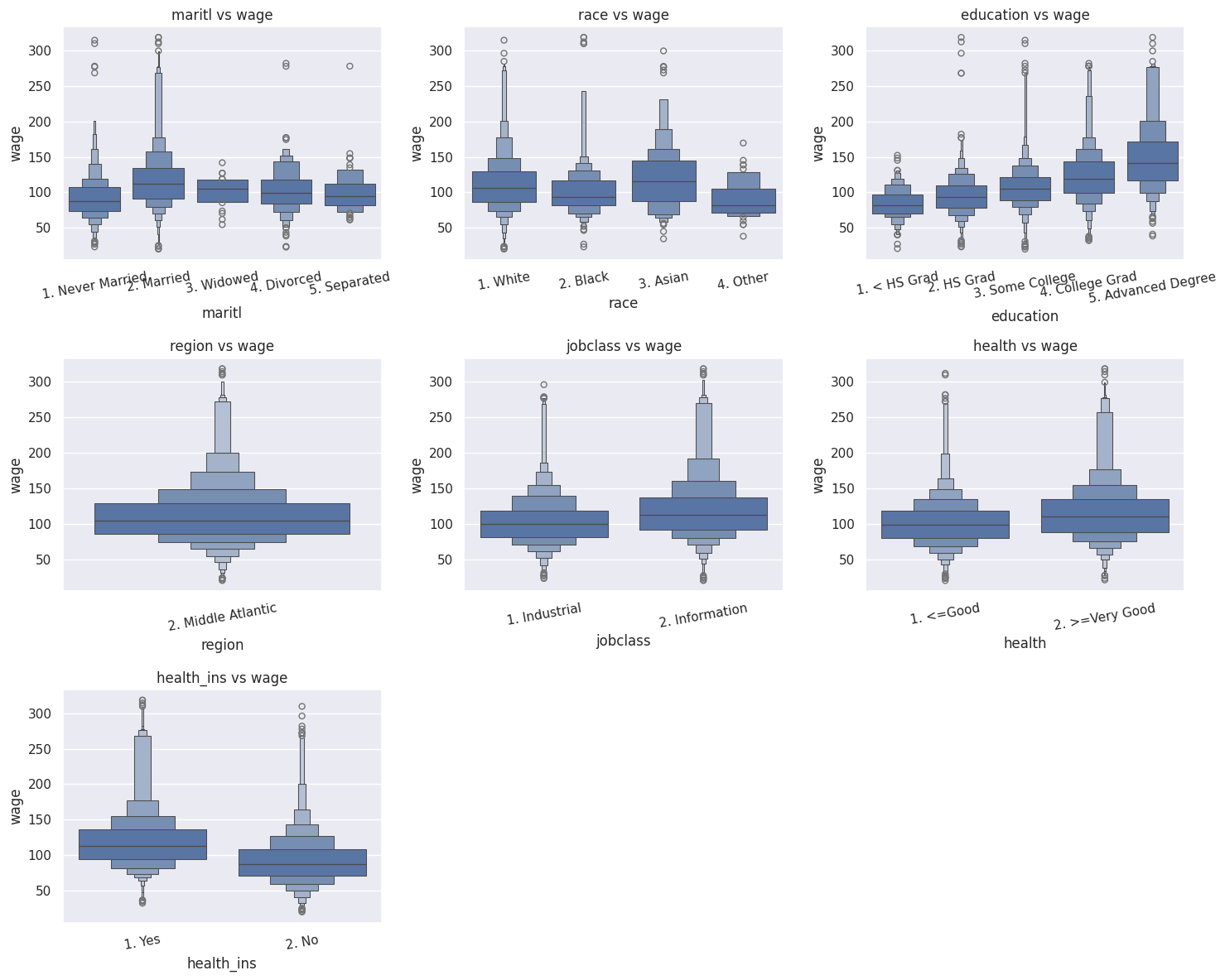
Some boxen plots of the qualitative variables.
categorical_columns = wage.select_dtypes(include=['object', 'category']).columns
categorical_columns
Index(['maritl', 'race', 'education', 'region', 'jobclass', 'health',
       'health_ins'],
      dtype='object')
n_cols = 3
n_rows = math.ceil(len(categorical_columns) / n_cols)

fig, axes = plt.subplots(n_rows, n_cols, figsize=(n_cols*5, n_rows*4), squeeze=False)
axes = axes.flatten()

for idx, col in enumerate(categorical_columns):
    sns.boxenplot(x=col, y='wage', data=wage, ax=axes[idx])
    axes[idx].set_title(f'{col} vs wage')
    axes[idx].tick_params(axis='x', labelrotation=10)
    axes[idx].tick_params(axis='y')

# If there are empty subplots, hide them
total_plots = n_rows * n_cols
for idx in range(len(categorical_columns), total_plots):
    axes[idx].set_visible(False)

plt.tight_layout()
def fit_gam(columns: list, df: pd.DataFrame) -> LinearGAM:
    """
    A simple function that fits gam models using factor terms with lam=0 for categorical variables
    and spline terms with default lam=0.6 for numerical variables.
    """
    cat_cols = df.select_dtypes(include=['object', 'category']).columns

    gam_terms = [f_gam(i, lam=0) if col in cat_cols else s_gam(i) for i, col in enumerate(columns)]
    X_terms = [df[col].cat.codes if col in cat_cols else df[col] for col in columns]

    gam = LinearGAM(np.sum(gam_terms))
    Xgam = np.column_stack(X_terms)
    return gam.fit(Xgam, y)


def plot_gam_terms(gam, columns: list, df:pd.DataFrame, y_name:str):
    """
    A simple function that plots partial gam plots on one figure
    """
    cat_cols = df.select_dtypes(include=['object', 'category']).columns

    n_plots = len(columns)
    n_rows = math.ceil(n_plots/3)
    n_cols = math.ceil(n_plots/n_rows)

    _, axes = plt.subplots(n_rows, n_cols, figsize=(n_cols*5, n_rows*4))
    axes = axes.flatten()

    for i, col in enumerate(columns):
        ax = axes[i]

        plot_gam(gam, i, ax=ax)

        ax.set_xlabel(col)
        ax.set_ylabel(f'Effect on {y_name}')
        ax.set_title(f'Partial dependence of {col} on {y_name}')

        if col in cat_cols:
            ax.set_xticklabels(df[col].cat.categories)
            ax.tick_params(axis='x', labelrotation=23)

    plt.tight_layout()
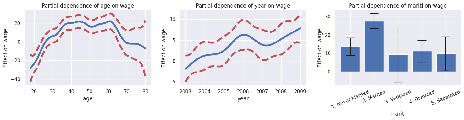
Now I’ll fit a bunch of GAM models using the functions defined above using different combinations of the columns
cols = ['age', 'year', 'maritl']
gam_maritl = fit_gam(cols, wage)
plot_gam_terms(gam_maritl, cols, wage, 'wage')
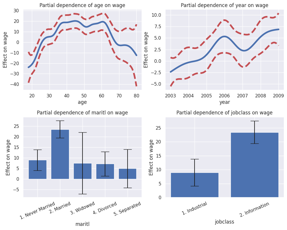
cols = ['age', 'year', 'maritl', 'jobclass']
gam_maritl_job = fit_gam(cols, wage)
plot_gam_terms(gam_maritl_job, cols, wage, 'wage')
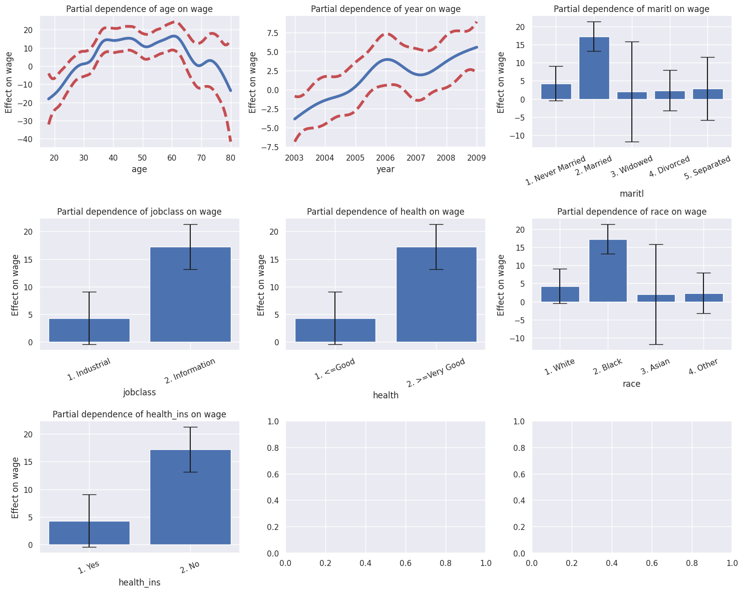
cols = ['age', 'year', 'maritl', 'jobclass', 'health', 'race', 'health_ins']
gam_full = fit_gam(cols, wage)
plot_gam_terms(gam_full, cols, wage, 'wage')
cols = ['age', 'year', 'race', 'jobclass', 'health', 'health_ins']
gam_no_maritl = fit_gam(cols, wage)
plot_gam_terms(gam_no_maritl, cols, wage, 'wage')
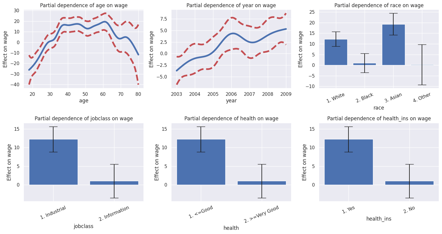
Removing the the maritl term significantly affected the other coefficients.
We’ll do a quick ANOVA test on the 3 models we fitted earlier.
Note: anova_gam assumes the models are nested, as in the predictors in the first model have to be a subset of the predictors in the second model and so on.
anova_gam(gam_maritl, gam_maritl_job, gam_full)
| deviance | df | deviance_diff | df_diff | F | pvalue | |
|---|---|---|---|---|---|---|
| 0 | 4.602715e+06 | 2974.804326 | NaN | NaN | NaN | NaN |
| 1 | 4.430372e+06 | 2973.804621 | 172343.496485 | 0.999705 | 126.804962 | 1.615249e-12 |
| 2 | 4.036164e+06 | 2968.807511 | 394207.280901 | 4.997110 | 58.025501 | 7.221814e-15 |
anova_gam(gam_no_maritl, gam_full)
| deviance | df | deviance_diff | df_diff | F | pvalue | |
|---|---|---|---|---|---|---|
| 0 | 4.133688e+06 | 2972.804219 | NaN | NaN | NaN | NaN |
| 1 | 4.036164e+06 | 2968.807511 | 97523.743223 | 3.996708 | 17.94821 | 9.697761e-08 |
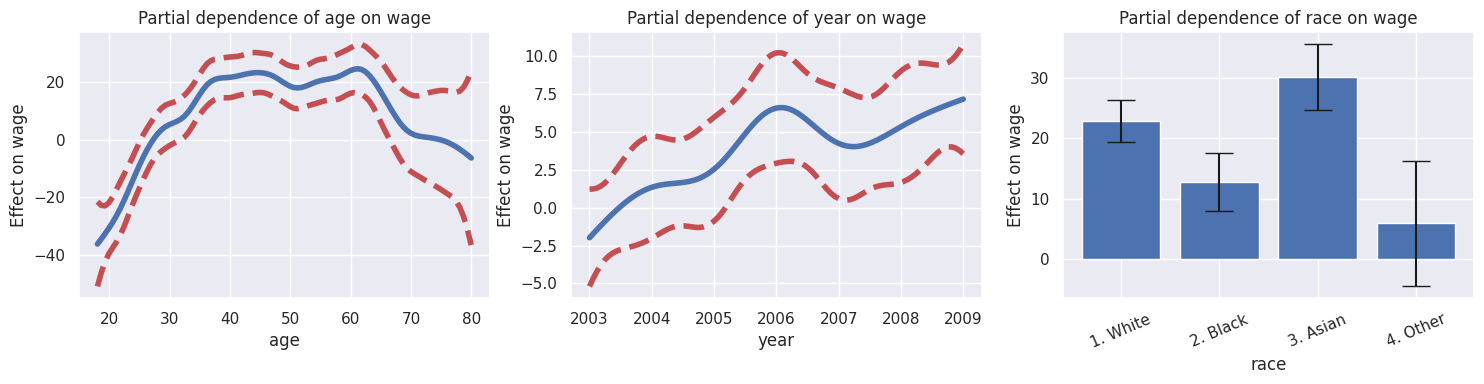
cols = ['age', 'year', 'race']
gam_race = fit_gam(cols, wage)
plot_gam_terms(gam_race, cols, wage, 'wage')
cols = ['age', 'year', 'race', 'health']
gam_health_race = fit_gam(cols, wage)
plot_gam_terms(gam_health_race, cols, wage, 'wage')
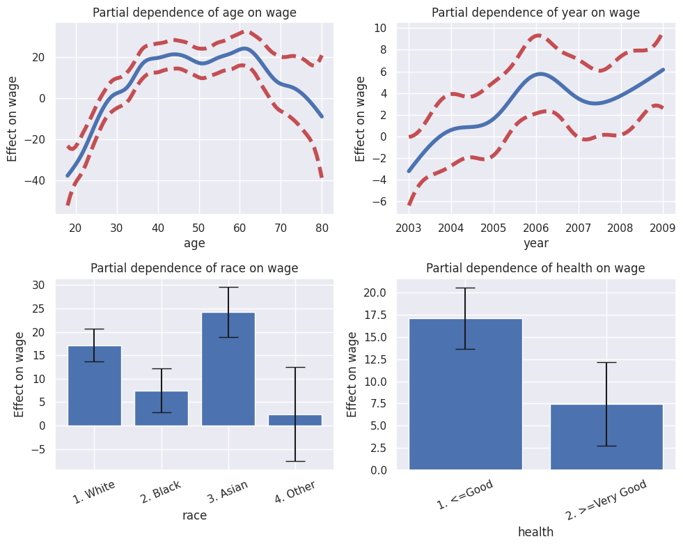
cols = ['age', 'year', 'maritl', 'jobclass', 'health', 'health_ins']
gam_no_race = fit_gam(cols, wage)
plot_gam_terms(gam_no_race, cols, wage, 'wage')
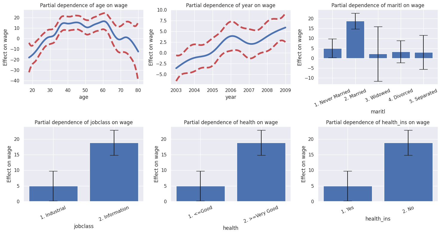
Comparing with the plot of gam_full from earlier we can see not much changed after removing the race predictor, this could indicate that most of the variance in wage is explained by the maritl predictor.
Another quick ANOVA test shows that while it’s not noticable in the plot the difference between the models is statistically significant.
anova_gam(gam_race, gam_health_race, gam_full)
| deviance | df | deviance_diff | df_diff | F | pvalue | |
|---|---|---|---|---|---|---|
| 0 | 4.676232e+06 | 2975.802852 | NaN | NaN | NaN | NaN |
| 1 | 4.538308e+06 | 2974.803262 | 137924.517292 | 0.999590 | 101.492259 | 2.517522e-11 |
| 2 | 4.036164e+06 | 2968.807511 | 502143.594980 | 5.995751 | 61.602383 | 6.406628e-16 |
anova_gam(gam_no_race, gam_full)
| deviance | df | deviance_diff | df_diff | F | pvalue | |
|---|---|---|---|---|---|---|
| 0 | 4.070757e+06 | 2971.805679 | NaN | NaN | NaN | NaN |
| 1 | 4.036164e+06 | 2968.807511 | 34593.144492 | 2.998168 | 8.486865 | 0.000288 |
Q8.#
auto = load_data('Auto')
auto.head()
| mpg | cylinders | displacement | horsepower | weight | acceleration | year | origin | |
|---|---|---|---|---|---|---|---|---|
| name | ||||||||
| chevrolet chevelle malibu | 18.0 | 8 | 307.0 | 130 | 3504 | 12.0 | 70 | 1 |
| buick skylark 320 | 15.0 | 8 | 350.0 | 165 | 3693 | 11.5 | 70 | 1 |
| plymouth satellite | 18.0 | 8 | 318.0 | 150 | 3436 | 11.0 | 70 | 1 |
| amc rebel sst | 16.0 | 8 | 304.0 | 150 | 3433 | 12.0 | 70 | 1 |
| ford torino | 17.0 | 8 | 302.0 | 140 | 3449 | 10.5 | 70 | 1 |
auto.info()
<class 'pandas.core.frame.DataFrame'>
Index: 392 entries, chevrolet chevelle malibu to chevy s-10
Data columns (total 8 columns):
 #   Column        Non-Null Count  Dtype
---  ------        --------------  -----
 0   mpg           392 non-null    float64
 1   cylinders     392 non-null    int64
 2   displacement  392 non-null    float64
 3   horsepower    392 non-null    int64
 4   weight        392 non-null    int64
 5   acceleration  392 non-null    float64
 6   year          392 non-null    int64
 7   origin        392 non-null    int64
dtypes: float64(3), int64(5)
memory usage: 27.6+ KB
auto.describe()
| mpg | cylinders | displacement | horsepower | weight | acceleration | year | origin | |
|---|---|---|---|---|---|---|---|---|
| count | 392.000000 | 392.000000 | 392.000000 | 392.000000 | 392.000000 | 392.000000 | 392.000000 | 392.000000 |
| mean | 23.445918 | 5.471939 | 194.411990 | 104.469388 | 2977.584184 | 15.541327 | 75.979592 | 1.576531 |
| std | 7.805007 | 1.705783 | 104.644004 | 38.491160 | 849.402560 | 2.758864 | 3.683737 | 0.805518 |
| min | 9.000000 | 3.000000 | 68.000000 | 46.000000 | 1613.000000 | 8.000000 | 70.000000 | 1.000000 |
| 25% | 17.000000 | 4.000000 | 105.000000 | 75.000000 | 2225.250000 | 13.775000 | 73.000000 | 1.000000 |
| 50% | 22.750000 | 4.000000 | 151.000000 | 93.500000 | 2803.500000 | 15.500000 | 76.000000 | 1.000000 |
| 75% | 29.000000 | 8.000000 | 275.750000 | 126.000000 | 3614.750000 | 17.025000 | 79.000000 | 2.000000 |
| max | 46.600000 | 8.000000 | 455.000000 | 230.000000 | 5140.000000 | 24.800000 | 82.000000 | 3.000000 |
g = sns.PairGrid(auto)
g.map_upper(plt.scatter, s=3)
g.map_diag(plt.hist)
g.map_lower(sns.kdeplot, cmap="Blues_d")
g.figure.set_size_inches(12, 12)
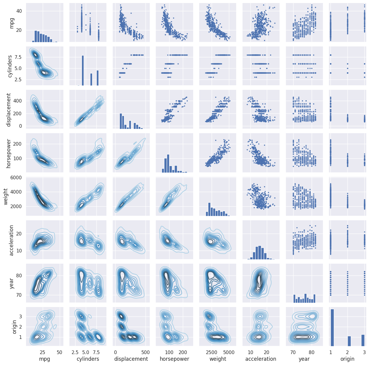
We can see some non-linear relationships for mpg.
plt.figure().set_size_inches(8, 8)
sns.heatmap(auto.corr(), annot=True, square=True);
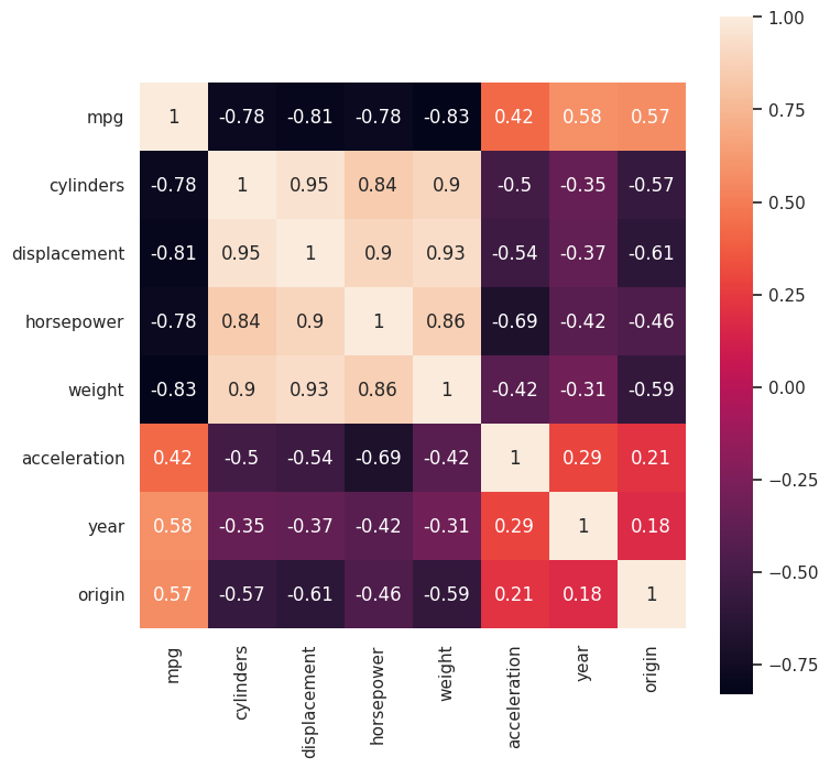
We’ll use the function we made earlier to make some GAM fits and plots.
def fit_gam(columns: list, df: pd.DataFrame, response: str, s_lam=0.6) -> LinearGAM:
    """
    A simple function that fits gam models using factor terms with lam=0 for categorical variables
    and spline terms with default lam=0.6 for numerical variables.
    """
    cat_cols = df.select_dtypes(include=['object', 'category']).columns

    gam_terms = [f_gam(i, lam=0) if col in cat_cols else s_gam(i, lam=s_lam) for i, col in enumerate(columns)]
    X_terms = [df[col].cat.codes if col in cat_cols else df[col] for col in columns]

    gam = LinearGAM(np.sum(gam_terms))
    Xgam = np.column_stack(X_terms)
    return gam.fit(Xgam, df[response])


def plot_gam_terms(gam, columns: list, df:pd.DataFrame, y_name:str):
    """
    A simple function that plots partial gam plots on one figure
    """
    cat_cols = df.select_dtypes(include=['object', 'category']).columns

    n_plots = len(columns)
    n_rows = math.ceil(n_plots/3)
    n_cols = math.ceil(n_plots/n_rows)

    _, axes = plt.subplots(n_rows, n_cols, figsize=(n_cols*5, n_rows*4))
    axes = axes.flatten()

    for i, col in enumerate(columns):
        ax = axes[i]

        plot_gam(gam, i, ax=ax)

        ax.set_xlabel(col)
        ax.set_ylabel(f'Effect on {y_name}')
        ax.set_title(f'Partial dependence of {col} on {y_name}')

        if col in cat_cols:
            ax.set_xticklabels(df[col].cat.categories)
            ax.tick_params(axis='x', labelrotation=23)

    plt.tight_layout()
cols = auto.columns.drop('mpg')
gam = fit_gam(cols, auto, response='mpg')
plot_gam_terms(gam, cols, auto, 'mpg')
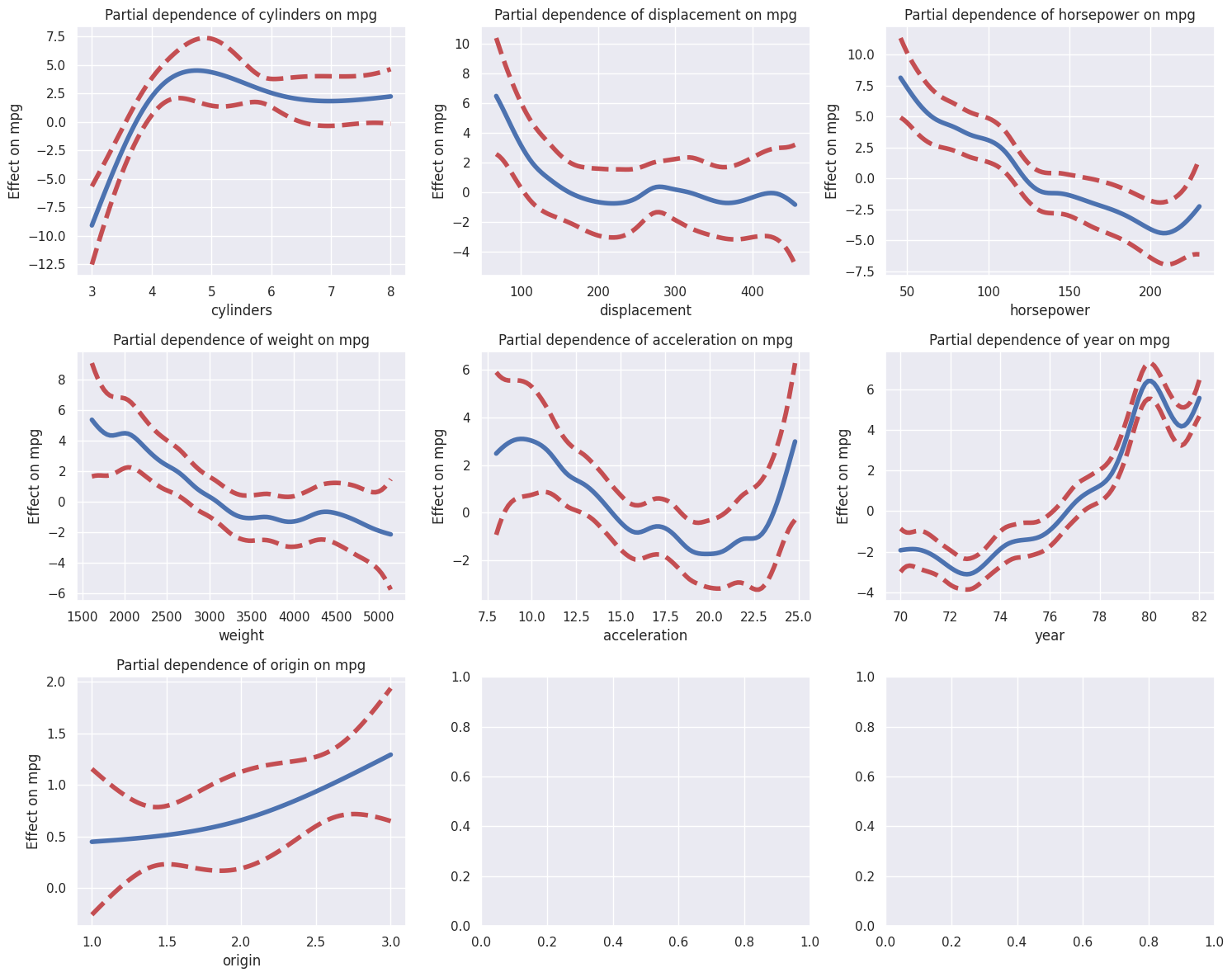
We’ll increase the value of the penalty lam to get smoother fits.
cols = auto.columns.drop('mpg')
gam = fit_gam(cols, auto, response='mpg', s_lam=70)
plot_gam_terms(gam, cols, auto, 'mpg')
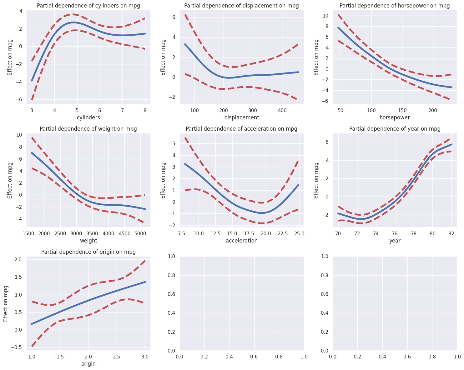
We can try a local regression (lowess) fit on the data too.
lowess = sm.nonparametric.lowess
fig, axes = plt.subplots(3, 3, figsize=(16,13))
axes = axes.flatten()
y = auto['mpg']

for i, col in enumerate(auto.columns.drop('mpg')):

    ax = axes[i]
    x_grid = np.linspace(auto[col].min(), auto[col].max(), 100)
    ax.scatter(auto[col], y, marker='o', facecolors='none', edgecolors='black', linewidths=0.6)

    for span in [0.65, 0.8, 1]:

        fitted = lowess(y,
                        auto[col],
                        frac=span,
                        xvals=x_grid)
        ax.plot(x_grid,
                fitted,
                label=f'{span:.2f}',
                linewidth=4,
                alpha=0.6)

    ax.set_xlabel(col, fontsize=13)
    ax.set_ylabel('mpg', fontsize=13);
    ax.legend(title='span', fontsize=12);

plt.tight_layout()
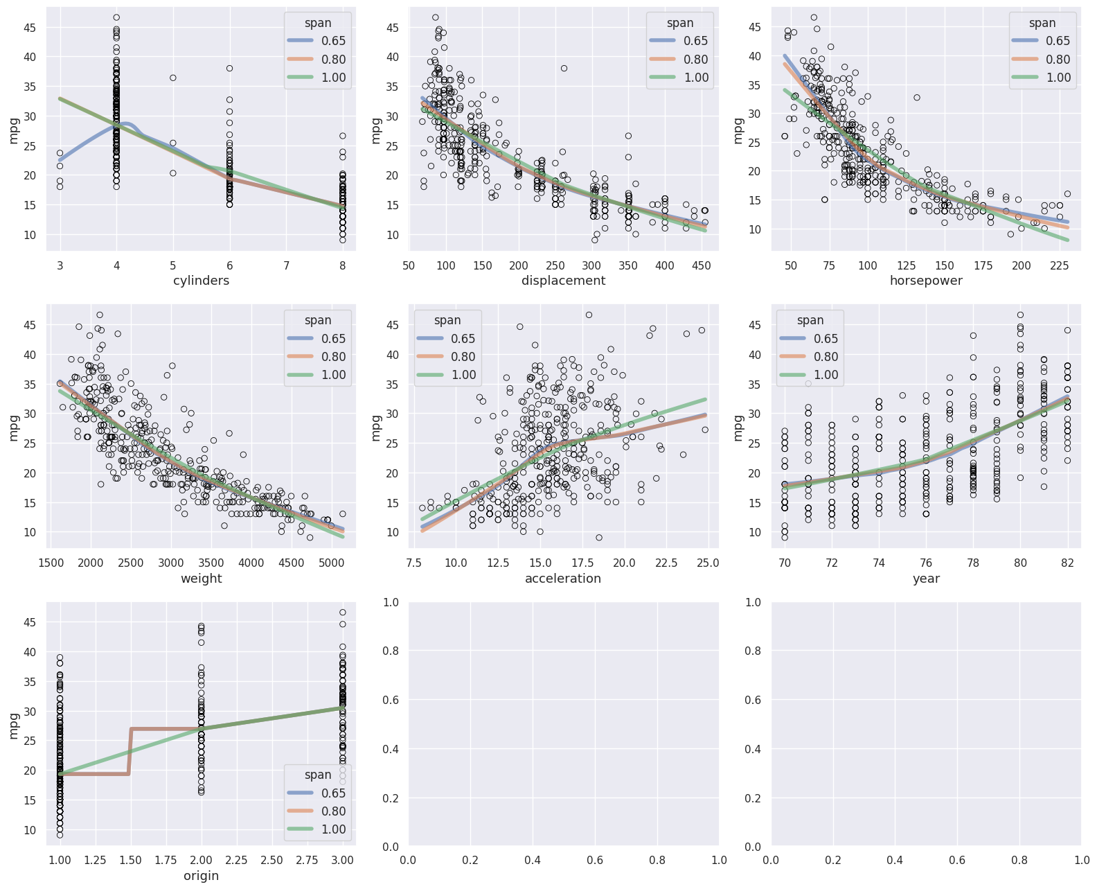
We can see that there’s a strong non-linear inverse relationship between mpg and predictors like displacement, horsepower, weight, And a slightly non-linear concave relationship between mpg and acceleration.
Q9.#
boston = load_data('Boston')
boston.head()
| crim | zn | indus | chas | nox | rm | age | dis | rad | tax | ptratio | lstat | medv | |
|---|---|---|---|---|---|---|---|---|---|---|---|---|---|
| 0 | 0.00632 | 18.0 | 2.31 | 0 | 0.538 | 6.575 | 65.2 | 4.0900 | 1 | 296 | 15.3 | 4.98 | 24.0 |
| 1 | 0.02731 | 0.0 | 7.07 | 0 | 0.469 | 6.421 | 78.9 | 4.9671 | 2 | 242 | 17.8 | 9.14 | 21.6 |
| 2 | 0.02729 | 0.0 | 7.07 | 0 | 0.469 | 7.185 | 61.1 | 4.9671 | 2 | 242 | 17.8 | 4.03 | 34.7 |
| 3 | 0.03237 | 0.0 | 2.18 | 0 | 0.458 | 6.998 | 45.8 | 6.0622 | 3 | 222 | 18.7 | 2.94 | 33.4 |
| 4 | 0.06905 | 0.0 | 2.18 | 0 | 0.458 | 7.147 | 54.2 | 6.0622 | 3 | 222 | 18.7 | 5.33 | 36.2 |
boston.describe(include='all')
| crim | zn | indus | chas | nox | rm | age | dis | rad | tax | ptratio | lstat | medv | |
|---|---|---|---|---|---|---|---|---|---|---|---|---|---|
| count | 506.000000 | 506.000000 | 506.000000 | 506.000000 | 506.000000 | 506.000000 | 506.000000 | 506.000000 | 506.000000 | 506.000000 | 506.000000 | 506.000000 | 506.000000 |
| mean | 3.613524 | 11.363636 | 11.136779 | 0.069170 | 0.554695 | 6.284634 | 68.574901 | 3.795043 | 9.549407 | 408.237154 | 18.455534 | 12.653063 | 22.532806 |
| std | 8.601545 | 23.322453 | 6.860353 | 0.253994 | 0.115878 | 0.702617 | 28.148861 | 2.105710 | 8.707259 | 168.537116 | 2.164946 | 7.141062 | 9.197104 |
| min | 0.006320 | 0.000000 | 0.460000 | 0.000000 | 0.385000 | 3.561000 | 2.900000 | 1.129600 | 1.000000 | 187.000000 | 12.600000 | 1.730000 | 5.000000 |
| 25% | 0.082045 | 0.000000 | 5.190000 | 0.000000 | 0.449000 | 5.885500 | 45.025000 | 2.100175 | 4.000000 | 279.000000 | 17.400000 | 6.950000 | 17.025000 |
| 50% | 0.256510 | 0.000000 | 9.690000 | 0.000000 | 0.538000 | 6.208500 | 77.500000 | 3.207450 | 5.000000 | 330.000000 | 19.050000 | 11.360000 | 21.200000 |
| 75% | 3.677083 | 12.500000 | 18.100000 | 0.000000 | 0.624000 | 6.623500 | 94.075000 | 5.188425 | 24.000000 | 666.000000 | 20.200000 | 16.955000 | 25.000000 |
| max | 88.976200 | 100.000000 | 27.740000 | 1.000000 | 0.871000 | 8.780000 | 100.000000 | 12.126500 | 24.000000 | 711.000000 | 22.000000 | 37.970000 | 50.000000 |
(a)
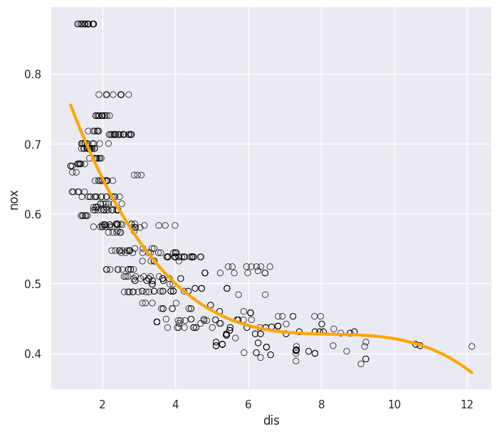
dis = boston['dis']
nox = boston['nox']
design = MS([poly('dis', degree=3)]).fit(boston)

X = design.transform(boston)
y = nox

results = sm.OLS(y, X).fit()
summarize(results)
| coef | std err | t | P>|t| | |
|---|---|---|---|---|
| intercept | 0.5547 | 0.003 | 201.021 | 0.0 |
| poly(dis, degree=3)[0] | -2.0031 | 0.062 | -32.271 | 0.0 |
| poly(dis, degree=3)[1] | 0.8563 | 0.062 | 13.796 | 0.0 |
| poly(dis, degree=3)[2] | -0.3180 | 0.062 | -5.124 | 0.0 |
fig, ax = plt.subplots(figsize=(8, 7))
x = dis
ax.scatter(x, y, marker='o', facecolors='none', edgecolors='black', linewidths=0.5)

xs = np.linspace(x.min(), x.max(), 1000)
xs_df = pd.DataFrame({'dis': xs})
ax.plot(xs, results.predict(design.transform(xs_df)), c='orange', lw=3)

ax.set_xlabel('dis')
ax.set_ylabel('nox');
(b) I’ll use sklearn’s Pipeline and PolynomialFeatures to fit the polynomials for degrees \(1, ..., 10\) since they’re more straighforward than poly and are easier to use with cross-validation.
print('\tTraining RSS')
rss = {}
for i in range(1, 11):

    pipe = Pipeline([('poly', PolynomialFeatures(degree=i)),
                    ('linreg', skl.LinearRegression())])
    x = np.reshape(dis, (-1, 1))
    results = pipe.fit(x, y)
    training_rss = np.sum((results.predict(x) - y)**2)
    print(f"degree {i}: {training_rss:0.4f}")
    rss[i] = training_rss

plt.plot(rss.keys(), rss.values(), 'r-o')
plt.xlabel('Polynomial Degree')
plt.ylabel('Training RSS');
	Training RSS
degree 1: 2.7686
degree 2: 2.0353
degree 3: 1.9341
degree 4: 1.9330
degree 5: 1.9153
degree 6: 1.8783
degree 7: 1.8495
degree 8: 1.8356
degree 9: 1.8333
degree 10: 1.8322
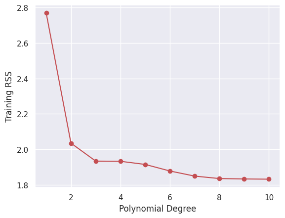
Not surprising that the most flexible model got the lowest training RSS.
(c) Now we’ll perform cross-validation to find the most optimal degree.
kfold = skm.KFold(5, shuffle=True, random_state=1)

pipe = Pipeline([('poly', PolynomialFeatures(degree=2)),
                ('linreg', skl.LinearRegression())])

x = np.reshape(dis, (-1, 1))

param_grid = {'poly__degree': np.arange(1, 20)}
grid = skm.GridSearchCV(pipe, param_grid=param_grid, cv=kfold)

results = grid.fit(x, y)
results
GridSearchCV(cv=KFold(n_splits=5, random_state=1, shuffle=True),
             estimator=Pipeline(steps=[('poly', PolynomialFeatures()),
                                       ('linreg', LinearRegression())]),
             param_grid={'poly__degree': array([ 1,  2,  3,  4,  5,  6,  7,  8,  9, 10, 11, 12, 13, 14, 15, 16, 17,
       18, 19])})
In a Jupyter environment, please rerun this cell to show the HTML representation or trust the notebook. On GitHub, the HTML representation is unable to render, please try loading this page with nbviewer.org.
GridSearchCV(cv=KFold(n_splits=5, random_state=1, shuffle=True),
             estimator=Pipeline(steps=[('poly', PolynomialFeatures()),
                                       ('linreg', LinearRegression())]),
             param_grid={'poly__degree': array([ 1,  2,  3,  4,  5,  6,  7,  8,  9, 10, 11, 12, 13, 14, 15, 16, 17,
18, 19])})Pipeline(steps=[('poly', PolynomialFeatures(degree=3)),
('linreg', LinearRegression())])PolynomialFeatures(degree=3)
LinearRegression()
results.best_params_
{'poly__degree': 3}
Cross-validation found the optimal degree to be \(3\) which is reasonable considering the plot from earlier (a) was a pretty good fit to the data with no big signs of overfitting.
(d)
x = dis

design = MS([bs('dis',
                 internal_knots=[(dis.max() -dis.min())/2],
                 degree=3)]).fit(boston)

X = design.transform(boston)
y = nox

results = sm.OLS(y, X).fit()
results.summary()
| Dep. Variable: | nox | R-squared: | 0.715 |
|---|---|---|---|
| Model: | OLS | Adj. R-squared: | 0.713 |
| Method: | Least Squares | F-statistic: | 314.3 |
| Date: | Sat, 05 Apr 2025 | Prob (F-statistic): | 4.83e-135 |
| Time: | 02:47:07 | Log-Likelihood: | 690.66 |
| No. Observations: | 506 | AIC: | -1371. |
| Df Residuals: | 501 | BIC: | -1350. |
| Df Model: | 4 | ||
| Covariance Type: | nonrobust |
| coef | std err | t | P>|t| | [0.025 | 0.975] | |
|---|---|---|---|---|---|---|
| intercept | 0.7596 | 0.011 | 71.651 | 0.000 | 0.739 | 0.780 |
| bs(dis, internal_knots=[5.49845], degree=3)[0] | -0.2104 | 0.023 | -9.252 | 0.000 | -0.255 | -0.166 |
| bs(dis, internal_knots=[5.49845], degree=3)[1] | -0.3793 | 0.025 | -15.218 | 0.000 | -0.428 | -0.330 |
| bs(dis, internal_knots=[5.49845], degree=3)[2] | -0.3183 | 0.041 | -7.839 | 0.000 | -0.398 | -0.239 |
| bs(dis, internal_knots=[5.49845], degree=3)[3] | -0.3693 | 0.050 | -7.425 | 0.000 | -0.467 | -0.272 |
| Omnibus: | 63.904 | Durbin-Watson: | 0.285 |
|---|---|---|---|
| Prob(Omnibus): | 0.000 | Jarque-Bera (JB): | 87.057 |
| Skew: | 0.912 | Prob(JB): | 1.25e-19 |
| Kurtosis: | 3.896 | Cond. No. | 23.0 |
Notes:
[1] Standard Errors assume that the covariance matrix of the errors is correctly specified.
fig, ax = plt.subplots(figsize=(8, 7))
x = dis
ax.scatter(x, y, marker='o', facecolors='none', edgecolors='black', linewidths=0.5)

xs = np.linspace(x.min(), x.max(), 1000)
xs_df = pd.DataFrame({'dis': xs})
ax.plot(xs, results.predict(design.transform(xs_df)), c='orange', lw=3)

ax.set_title('Cubic Spline')
ax.set_xlabel('dis')
ax.set_ylabel('nox');
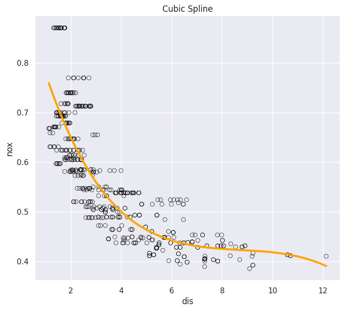
I chose one knot in the middle of the range to get 4 degrees of freedom.
The knot is at the following point:
(dis.max() -dis.min())/2
5.49845
(e)
print('\t\tTraining RSS')
results_dict = {}
for i in range(3, 12):

    design = MS([bs('dis',
                    df=i,
                    degree=3)]).fit(boston)

    X = design.transform(boston)
    y = nox

    results = sm.OLS(y, X).fit()

    training_rss = np.sum((results.predict(X) - y)**2)
    print(f"degree of freedom {i}: {training_rss:0.4f}")
    results_dict[i] = (design, results, training_rss)

rss_values = [value[2] for value in results_dict.values()]
plt.plot(results_dict.keys(), rss_values, 'r-o')
plt.xlabel('degree of freedom')
plt.ylabel('Training RSS');
		Training RSS
degree of freedom 3: 1.9341
degree of freedom 4: 1.9228
degree of freedom 5: 1.8402
degree of freedom 6: 1.8340
degree of freedom 7: 1.8299
degree of freedom 8: 1.8170
degree of freedom 9: 1.8257
degree of freedom 10: 1.7925
degree of freedom 11: 1.7970
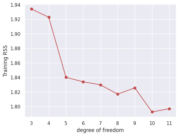
fig, axes = plt.subplots(3, 3, figsize=(14, 14))
axes = axes.flatten()

x = dis
xs = np.linspace(x.min(), x.max(), 1000)
xs_df = pd.DataFrame({'dis': xs})

for idx, value in results_dict.items():
    design, model, _ = value
    ax = axes[idx-3]

    ax.scatter(x, y, marker='o', facecolors='none', edgecolors='black', linewidths=0.5)
    ax.plot(xs, model.predict(design.transform(xs_df)), c='orange', lw=3)

    ax.set_title(f'Cubic Spline df = {idx}')
    ax.set_xlabel('dis')
    ax.set_ylabel('nox')
    plt.tight_layout();
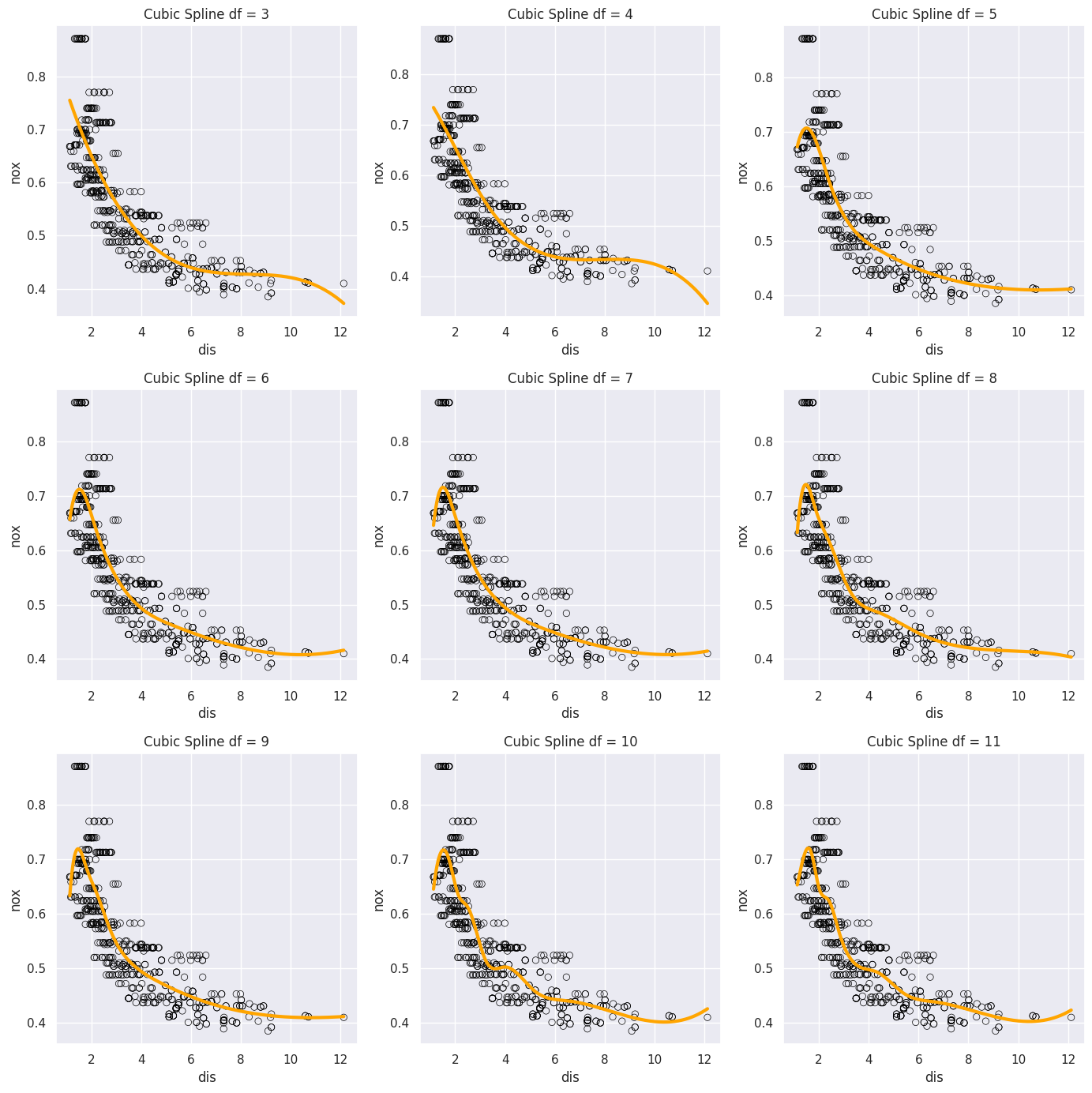
We can see that the model starts overfitting to the beginning of the data pretty quickly as the degrees of freedom increase.
(f) Again for cross-validation I’ll use the sklearn implementation since it’s more straightforward.
kfold = skm.KFold(7, shuffle=True, random_state=1)

pipe = Pipeline([('spline', SplineTransformer(n_knots=2, degree=3, knots='quantile')),
                ('linreg', skl.LinearRegression())])

x = np.reshape(dis, (-1, 1))

param_grid = {'spline__degree': np.arange(1, 20),
            'spline__n_knots': np.arange(2, 20)}

grid = skm.GridSearchCV(pipe, param_grid=param_grid, cv=kfold)

results = grid.fit(x, y)
results
GridSearchCV(cv=KFold(n_splits=7, random_state=1, shuffle=True),
             estimator=Pipeline(steps=[('spline',
                                        SplineTransformer(knots='quantile',
                                                          n_knots=2)),
                                       ('linreg', LinearRegression())]),
             param_grid={'spline__degree': array([ 1,  2,  3,  4,  5,  6,  7,  8,  9, 10, 11, 12, 13, 14, 15, 16, 17,
       18, 19]),
                         'spline__n_knots': array([ 2,  3,  4,  5,  6,  7,  8,  9, 10, 11, 12, 13, 14, 15, 16, 17, 18,
       19])})
In a Jupyter environment, please rerun this cell to show the HTML representation or trust the notebook. On GitHub, the HTML representation is unable to render, please try loading this page with nbviewer.org.
GridSearchCV(cv=KFold(n_splits=7, random_state=1, shuffle=True),
             estimator=Pipeline(steps=[('spline',
                                        SplineTransformer(knots='quantile',
                                                          n_knots=2)),
                                       ('linreg', LinearRegression())]),
             param_grid={'spline__degree': array([ 1,  2,  3,  4,  5,  6,  7,  8,  9, 10, 11, 12, 13, 14, 15, 16, 17,
       18, 19]),
                         'spline__n_knots': array([ 2,  3,  4,  5,  6,  7,  8,  9, 10, 11, 12, 13, 14, 15, 16, 17, 18,
19])})Pipeline(steps=[('spline',
SplineTransformer(degree=2, knots='quantile', n_knots=8)),
('linreg', LinearRegression())])SplineTransformer(degree=2, knots='quantile', n_knots=8)
LinearRegression()
best_estimator = results.best_estimator_
results.best_params_
{'spline__degree': 2, 'spline__n_knots': 8}
fig, ax = plt.subplots(figsize=(8, 7))
x = dis
ax.scatter(x, y, marker='o', facecolors='none', edgecolors='black', linewidths=0.5)

xs = np.linspace(x.min(), x.max(), 1000).reshape(-1, 1)
ax.plot(xs, best_estimator.predict(xs), c='orange', lw=3)

ax.set_title('Cubic Spline')
ax.set_xlabel('dis')
ax.set_ylabel('nox');
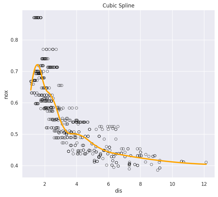
Cross-validation picked the estimator with degree=2 and n_knots=8, which is \(3+ \text{n\_knots} = 8\) degrees of freedom.
Q10.#
college = load_data('College')
college.head()
| Private | Apps | Accept | Enroll | Top10perc | Top25perc | F.Undergrad | P.Undergrad | Outstate | Room.Board | Books | Personal | PhD | Terminal | S.F.Ratio | perc.alumni | Expend | Grad.Rate | |
|---|---|---|---|---|---|---|---|---|---|---|---|---|---|---|---|---|---|---|
| 0 | Yes | 1660 | 1232 | 721 | 23 | 52 | 2885 | 537 | 7440 | 3300 | 450 | 2200 | 70 | 78 | 18.1 | 12 | 7041 | 60 |
| 1 | Yes | 2186 | 1924 | 512 | 16 | 29 | 2683 | 1227 | 12280 | 6450 | 750 | 1500 | 29 | 30 | 12.2 | 16 | 10527 | 56 |
| 2 | Yes | 1428 | 1097 | 336 | 22 | 50 | 1036 | 99 | 11250 | 3750 | 400 | 1165 | 53 | 66 | 12.9 | 30 | 8735 | 54 |
| 3 | Yes | 417 | 349 | 137 | 60 | 89 | 510 | 63 | 12960 | 5450 | 450 | 875 | 92 | 97 | 7.7 | 37 | 19016 | 59 |
| 4 | Yes | 193 | 146 | 55 | 16 | 44 | 249 | 869 | 7560 | 4120 | 800 | 1500 | 76 | 72 | 11.9 | 2 | 10922 | 15 |
college.info()
<class 'pandas.core.frame.DataFrame'>
RangeIndex: 777 entries, 0 to 776
Data columns (total 18 columns):
 #   Column       Non-Null Count  Dtype
---  ------       --------------  -----
 0   Private      777 non-null    category
 1   Apps         777 non-null    int64
 2   Accept       777 non-null    int64
 3   Enroll       777 non-null    int64
 4   Top10perc    777 non-null    int64
 5   Top25perc    777 non-null    int64
 6   F.Undergrad  777 non-null    int64
 7   P.Undergrad  777 non-null    int64
 8   Outstate     777 non-null    int64
 9   Room.Board   777 non-null    int64
 10  Books        777 non-null    int64
 11  Personal     777 non-null    int64
 12  PhD          777 non-null    int64
 13  Terminal     777 non-null    int64
 14  S.F.Ratio    777 non-null    float64
 15  perc.alumni  777 non-null    int64
 16  Expend       777 non-null    int64
 17  Grad.Rate    777 non-null    int64
dtypes: category(1), float64(1), int64(16)
memory usage: 104.2 KB
college.describe(include='category')
| Private | |
|---|---|
| count | 777 |
| unique | 2 |
| top | Yes |
| freq | 565 |
college.describe()
| Apps | Accept | Enroll | Top10perc | Top25perc | F.Undergrad | P.Undergrad | Outstate | Room.Board | Books | Personal | PhD | Terminal | S.F.Ratio | perc.alumni | Expend | Grad.Rate | |
|---|---|---|---|---|---|---|---|---|---|---|---|---|---|---|---|---|---|
| count | 777.000000 | 777.000000 | 777.000000 | 777.000000 | 777.000000 | 777.000000 | 777.000000 | 777.000000 | 777.000000 | 777.000000 | 777.000000 | 777.000000 | 777.000000 | 777.000000 | 777.000000 | 777.000000 | 777.00000 |
| mean | 3001.638353 | 2018.804376 | 779.972973 | 27.558559 | 55.796654 | 3699.907336 | 855.298584 | 10440.669241 | 4357.526384 | 549.380952 | 1340.642214 | 72.660232 | 79.702703 | 14.089704 | 22.743887 | 9660.171171 | 65.46332 |
| std | 3870.201484 | 2451.113971 | 929.176190 | 17.640364 | 19.804778 | 4850.420531 | 1522.431887 | 4023.016484 | 1096.696416 | 165.105360 | 677.071454 | 16.328155 | 14.722359 | 3.958349 | 12.391801 | 5221.768440 | 17.17771 |
| min | 81.000000 | 72.000000 | 35.000000 | 1.000000 | 9.000000 | 139.000000 | 1.000000 | 2340.000000 | 1780.000000 | 96.000000 | 250.000000 | 8.000000 | 24.000000 | 2.500000 | 0.000000 | 3186.000000 | 10.00000 |
| 25% | 776.000000 | 604.000000 | 242.000000 | 15.000000 | 41.000000 | 992.000000 | 95.000000 | 7320.000000 | 3597.000000 | 470.000000 | 850.000000 | 62.000000 | 71.000000 | 11.500000 | 13.000000 | 6751.000000 | 53.00000 |
| 50% | 1558.000000 | 1110.000000 | 434.000000 | 23.000000 | 54.000000 | 1707.000000 | 353.000000 | 9990.000000 | 4200.000000 | 500.000000 | 1200.000000 | 75.000000 | 82.000000 | 13.600000 | 21.000000 | 8377.000000 | 65.00000 |
| 75% | 3624.000000 | 2424.000000 | 902.000000 | 35.000000 | 69.000000 | 4005.000000 | 967.000000 | 12925.000000 | 5050.000000 | 600.000000 | 1700.000000 | 85.000000 | 92.000000 | 16.500000 | 31.000000 | 10830.000000 | 78.00000 |
| max | 48094.000000 | 26330.000000 | 6392.000000 | 96.000000 | 100.000000 | 31643.000000 | 21836.000000 | 21700.000000 | 8124.000000 | 2340.000000 | 6800.000000 | 103.000000 | 100.000000 | 39.800000 | 64.000000 | 56233.000000 | 118.00000 |
We’ll turn the Private column to a boolean so it works with the ISLP methods below.
college['Private'] = college['Private'] == 'Yes'
(a)
Now to perform forward stepwise selection we’ll use Stepwise and sklearn_selected from the ISLP package with negative \(C_p\) as a scorer.
def nCp(sigma2, estimator, X, Y):
    "Negative Cp statistic"
    n, p = X.shape
    Yhat = estimator.predict(X)
    RSS = np.sum((Y - Yhat)**2)
    return -(RSS + 2 * p * sigma2) / n
design = MS(college.columns.drop('Outstate'))
X = design.fit_transform(college)
y = college['Outstate']
X_train, X_test, y_train, y_test = skm.train_test_split(X, y, test_size=0.3, random_state=1)
We’ll use the training data to estimate the variance needed to calculate negative \(C_p\).
sigma2 = sm.OLS(y_train, X_train).fit().scale
neg_Cp = partial(nCp, sigma2)
strategy = Stepwise.first_peak(design,
                               direction='forward',
                               max_terms=len(design.terms),
                               random_state=1)
college_selected = sklearn_selected(sm.OLS,
                                    strategy,
                                    scoring=neg_Cp)
college_selected.fit(X_train, y_train)
college_selected.selected_state_
('Accept',
 'Apps',
 'Enroll',
 'Expend',
 'Grad.Rate',
 'Personal',
 'PhD',
 'Private',
 'Room.Board',
 'S.F.Ratio',
 'Top10perc',
 'Top25perc',
 'perc.alumni')
selected_columns = list(college_selected.selected_state_)
These are the predictors selected by forward stepwise selection.
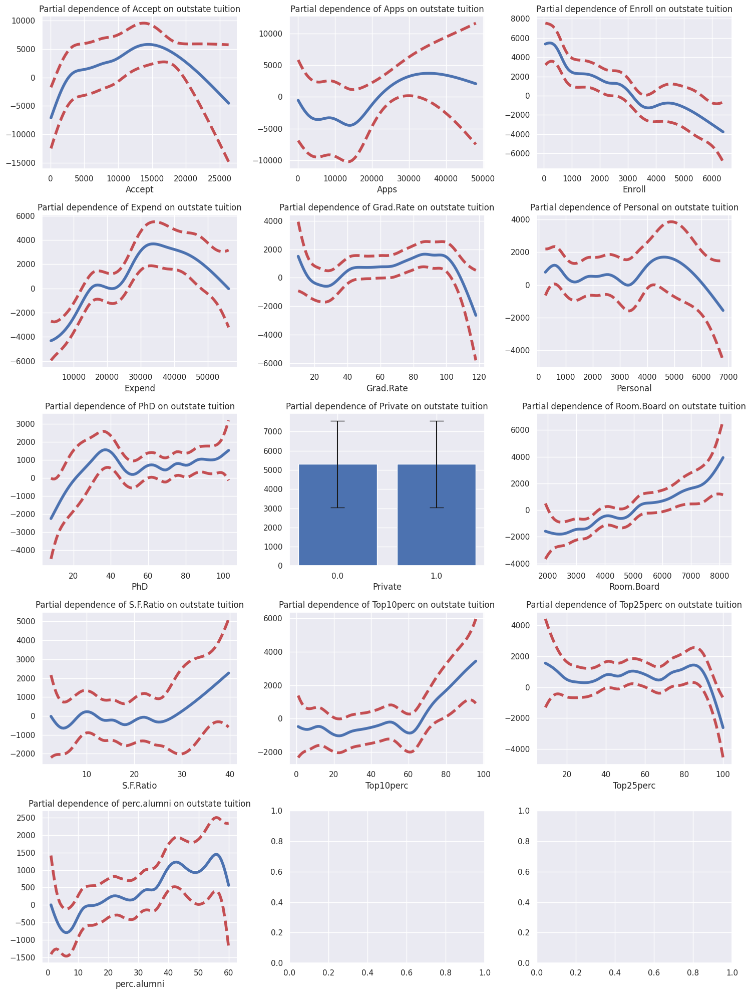
(b) Now we’ll fit a GAM model to the selected features with a factor term for the Private predictor since it’s categorical and 12 spline terms for the other predictors.
gam = LinearGAM(s_gam(0) +
                s_gam(1) +
                s_gam(2) +
                s_gam(3) +
                s_gam(4) +
                s_gam(5) +
                s_gam(6) +
                f_gam(7, lam=0) +
                s_gam(8) +
                s_gam(9) +
                s_gam(10) +
                s_gam(11) +
                s_gam(12))
gam.fit(X_train[selected_columns], y_train)
LinearGAM(callbacks=[Deviance(), Diffs()], fit_intercept=True,
   max_iter=100, scale=None,
   terms=s(0) + s(1) + s(2) + s(3) + s(4) + s(5) + s(6) + f(7) + s(8) + s(9) + s(10) + s(11) + s(12) + intercept,
   tol=0.0001, verbose=False)
I picked these penalty values after a few fits and decided that some curves could use some smoothing out.
n_plots = len(selected_columns)
n_rows = math.ceil(n_plots/3)
n_cols = math.ceil(n_plots/n_rows)

fig, axes = plt.subplots(n_rows, n_cols, figsize=(n_cols*5, n_rows*4))
axes = axes.flatten()

for i, col in enumerate(selected_columns):
    ax = axes[i]

    plot_gam(gam, i, ax=ax)

    ax.set_xlabel(col)
    ax.set_title(f'Partial dependence of {col} on outstate tuition')

plt.tight_layout()
(c) We’ll evaluate model performance by calculating the RMSE.
rmse = np.sqrt(np.mean((y_test - gam.predict(X_test[selected_columns]))**2))
rmse
1914.681341985242
college['Outstate'].mean(), college['Outstate'].std()
(10440.66924066924, 4023.016484111974)
We can see that our model makes pretty good predictions that fall within \(0.5\sigma\).
rmse/college['Outstate'].std()
0.47593176651074093
(d)
The non-linear relationship seems to be most pronounced for the variables Expend, PhD, Grad.Rate, Accept.
Q11.#
(a)
rng = np.random.default_rng(5)
x1 = rng.normal(0, 1, 100)
x2 = rng.normal(0, 1, 100)
eps = rng.normal(0, 10, 100)
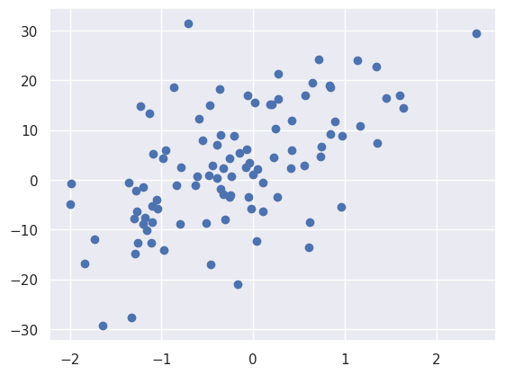
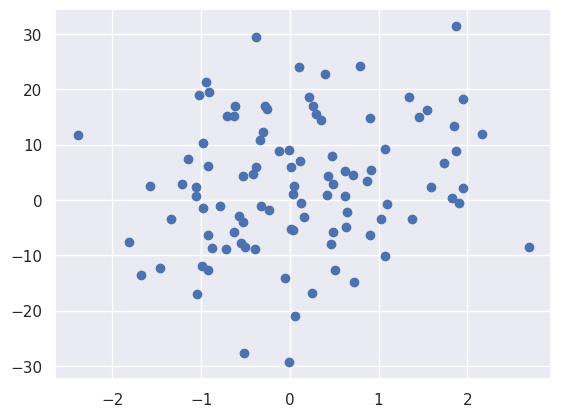
y =  4 + 7 * x1 + 2.5 * x2 + eps
plt.scatter(x1, y);
plt.scatter(x2, y);
(b)
def simple_reg(outcome, feature):
    y = outcome
    x = feature

    beta1 = sum((x - x.mean()) * (y - y.mean()))/(np.sum((x - x.mean())**2))
    beta0 = y.mean() - beta1 * x.mean()

    return beta0, beta1
(c)
beta1 = 2
(d)
beta0, beta2 = simple_reg(y - beta1 * x1, x2)
beta0, beta2
(3.0020617834203165, 2.1940648698152145)
(e)
beta0, beta1 = simple_reg(y - beta2 * x2, x1)
beta0, beta1
(4.307932494470254, 7.82959083901761)
(f) I believe the question means to repeat (d) and (e) not (c) and (d) for a thousand iterations as (c) just initiliazes a value for beta1.
iter_dict = {}
beta0 = beta1 = beta2 = 0
for i in range(1000):
    beta0, beta2 = simple_reg(y - beta1 * x1, x2)
    beta0, beta1 = simple_reg(y - beta2 * x2, x1)
    # if i % 10 ==0:
    iter_dict[i] = [beta0, beta1, beta2]
    print(f"iter {i}: {beta0}, {beta1}, {beta2}")

beta0, beta1, beta2
iter 0: 4.317527003764373, 7.819020992890909, 2.0670041568030446
iter 1: 4.280017168970773, 7.860343917269069, 2.563749348009967
iter 2: 4.2798189323797695, 7.860562305745158, 2.5663746081275867
iter 3: 4.279817884714638, 7.860563459911453, 2.566388482425328
iter 4: 4.279817879177808, 7.860563466011133, 2.5663885557499246
iter 5: 4.279817879148546, 7.860563466043369, 2.566388556137441
iter 6: 4.279817879148392, 7.860563466043541, 2.5663885561394872
iter 7: 4.279817879148391, 7.860563466043541, 2.5663885561394992
iter 8: 4.279817879148391, 7.860563466043541, 2.5663885561394992
iter 9: 4.279817879148391, 7.860563466043541, 2.5663885561394992
iter 10: 4.279817879148391, 7.860563466043541, 2.5663885561394992
iter 11: 4.279817879148391, 7.860563466043541, 2.5663885561394992
iter 12: 4.279817879148391, 7.860563466043541, 2.5663885561394992
iter 13: 4.279817879148391, 7.860563466043541, 2.5663885561394992
iter 14: 4.279817879148391, 7.860563466043541, 2.5663885561394992
iter 15: 4.279817879148391, 7.860563466043541, 2.5663885561394992
iter 16: 4.279817879148391, 7.860563466043541, 2.5663885561394992
iter 17: 4.279817879148391, 7.860563466043541, 2.5663885561394992
iter 18: 4.279817879148391, 7.860563466043541, 2.5663885561394992
iter 19: 4.279817879148391, 7.860563466043541, 2.5663885561394992
iter 20: 4.279817879148391, 7.860563466043541, 2.5663885561394992
iter 21: 4.279817879148391, 7.860563466043541, 2.5663885561394992
iter 22: 4.279817879148391, 7.860563466043541, 2.5663885561394992
iter 23: 4.279817879148391, 7.860563466043541, 2.5663885561394992
iter 24: 4.279817879148391, 7.860563466043541, 2.5663885561394992
iter 25: 4.279817879148391, 7.860563466043541, 2.5663885561394992
iter 26: 4.279817879148391, 7.860563466043541, 2.5663885561394992
iter 27: 4.279817879148391, 7.860563466043541, 2.5663885561394992
iter 28: 4.279817879148391, 7.860563466043541, 2.5663885561394992
iter 29: 4.279817879148391, 7.860563466043541, 2.5663885561394992
iter 30: 4.279817879148391, 7.860563466043541, 2.5663885561394992
iter 31: 4.279817879148391, 7.860563466043541, 2.5663885561394992
iter 32: 4.279817879148391, 7.860563466043541, 2.5663885561394992
iter 33: 4.279817879148391, 7.860563466043541, 2.5663885561394992
iter 34: 4.279817879148391, 7.860563466043541, 2.5663885561394992
iter 35: 4.279817879148391, 7.860563466043541, 2.5663885561394992
iter 36: 4.279817879148391, 7.860563466043541, 2.5663885561394992
iter 37: 4.279817879148391, 7.860563466043541, 2.5663885561394992
iter 38: 4.279817879148391, 7.860563466043541, 2.5663885561394992
iter 39: 4.279817879148391, 7.860563466043541, 2.5663885561394992
iter 40: 4.279817879148391, 7.860563466043541, 2.5663885561394992
iter 41: 4.279817879148391, 7.860563466043541, 2.5663885561394992
iter 42: 4.279817879148391, 7.860563466043541, 2.5663885561394992
iter 43: 4.279817879148391, 7.860563466043541, 2.5663885561394992
iter 44: 4.279817879148391, 7.860563466043541, 2.5663885561394992
iter 45: 4.279817879148391, 7.860563466043541, 2.5663885561394992
iter 46: 4.279817879148391, 7.860563466043541, 2.5663885561394992
iter 47: 4.279817879148391, 7.860563466043541, 2.5663885561394992
iter 48: 4.279817879148391, 7.860563466043541, 2.5663885561394992
iter 49: 4.279817879148391, 7.860563466043541, 2.5663885561394992
iter 50: 4.279817879148391, 7.860563466043541, 2.5663885561394992
iter 51: 4.279817879148391, 7.860563466043541, 2.5663885561394992
iter 52: 4.279817879148391, 7.860563466043541, 2.5663885561394992
iter 53: 4.279817879148391, 7.860563466043541, 2.5663885561394992
iter 54: 4.279817879148391, 7.860563466043541, 2.5663885561394992
iter 55: 4.279817879148391, 7.860563466043541, 2.5663885561394992
iter 56: 4.279817879148391, 7.860563466043541, 2.5663885561394992
iter 57: 4.279817879148391, 7.860563466043541, 2.5663885561394992
iter 58: 4.279817879148391, 7.860563466043541, 2.5663885561394992
iter 59: 4.279817879148391, 7.860563466043541, 2.5663885561394992
iter 60: 4.279817879148391, 7.860563466043541, 2.5663885561394992
iter 61: 4.279817879148391, 7.860563466043541, 2.5663885561394992
iter 62: 4.279817879148391, 7.860563466043541, 2.5663885561394992
iter 63: 4.279817879148391, 7.860563466043541, 2.5663885561394992
iter 64: 4.279817879148391, 7.860563466043541, 2.5663885561394992
iter 65: 4.279817879148391, 7.860563466043541, 2.5663885561394992
iter 66: 4.279817879148391, 7.860563466043541, 2.5663885561394992
iter 67: 4.279817879148391, 7.860563466043541, 2.5663885561394992
iter 68: 4.279817879148391, 7.860563466043541, 2.5663885561394992
iter 69: 4.279817879148391, 7.860563466043541, 2.5663885561394992
iter 70: 4.279817879148391, 7.860563466043541, 2.5663885561394992
iter 71: 4.279817879148391, 7.860563466043541, 2.5663885561394992
iter 72: 4.279817879148391, 7.860563466043541, 2.5663885561394992
iter 73: 4.279817879148391, 7.860563466043541, 2.5663885561394992
iter 74: 4.279817879148391, 7.860563466043541, 2.5663885561394992
iter 75: 4.279817879148391, 7.860563466043541, 2.5663885561394992
iter 76: 4.279817879148391, 7.860563466043541, 2.5663885561394992
iter 77: 4.279817879148391, 7.860563466043541, 2.5663885561394992
iter 78: 4.279817879148391, 7.860563466043541, 2.5663885561394992
iter 79: 4.279817879148391, 7.860563466043541, 2.5663885561394992
iter 80: 4.279817879148391, 7.860563466043541, 2.5663885561394992
iter 81: 4.279817879148391, 7.860563466043541, 2.5663885561394992
iter 82: 4.279817879148391, 7.860563466043541, 2.5663885561394992
iter 83: 4.279817879148391, 7.860563466043541, 2.5663885561394992
iter 84: 4.279817879148391, 7.860563466043541, 2.5663885561394992
iter 85: 4.279817879148391, 7.860563466043541, 2.5663885561394992
iter 86: 4.279817879148391, 7.860563466043541, 2.5663885561394992
iter 87: 4.279817879148391, 7.860563466043541, 2.5663885561394992
iter 88: 4.279817879148391, 7.860563466043541, 2.5663885561394992
iter 89: 4.279817879148391, 7.860563466043541, 2.5663885561394992
iter 90: 4.279817879148391, 7.860563466043541, 2.5663885561394992
iter 91: 4.279817879148391, 7.860563466043541, 2.5663885561394992
iter 92: 4.279817879148391, 7.860563466043541, 2.5663885561394992
iter 93: 4.279817879148391, 7.860563466043541, 2.5663885561394992
iter 94: 4.279817879148391, 7.860563466043541, 2.5663885561394992
iter 95: 4.279817879148391, 7.860563466043541, 2.5663885561394992
iter 96: 4.279817879148391, 7.860563466043541, 2.5663885561394992
iter 97: 4.279817879148391, 7.860563466043541, 2.5663885561394992
iter 98: 4.279817879148391, 7.860563466043541, 2.5663885561394992
iter 99: 4.279817879148391, 7.860563466043541, 2.5663885561394992
iter 100: 4.279817879148391, 7.860563466043541, 2.5663885561394992
iter 101: 4.279817879148391, 7.860563466043541, 2.5663885561394992
iter 102: 4.279817879148391, 7.860563466043541, 2.5663885561394992
iter 103: 4.279817879148391, 7.860563466043541, 2.5663885561394992
iter 104: 4.279817879148391, 7.860563466043541, 2.5663885561394992
iter 105: 4.279817879148391, 7.860563466043541, 2.5663885561394992
iter 106: 4.279817879148391, 7.860563466043541, 2.5663885561394992
iter 107: 4.279817879148391, 7.860563466043541, 2.5663885561394992
iter 108: 4.279817879148391, 7.860563466043541, 2.5663885561394992
iter 109: 4.279817879148391, 7.860563466043541, 2.5663885561394992
iter 110: 4.279817879148391, 7.860563466043541, 2.5663885561394992
iter 111: 4.279817879148391, 7.860563466043541, 2.5663885561394992
iter 112: 4.279817879148391, 7.860563466043541, 2.5663885561394992
iter 113: 4.279817879148391, 7.860563466043541, 2.5663885561394992
iter 114: 4.279817879148391, 7.860563466043541, 2.5663885561394992
iter 115: 4.279817879148391, 7.860563466043541, 2.5663885561394992
iter 116: 4.279817879148391, 7.860563466043541, 2.5663885561394992
iter 117: 4.279817879148391, 7.860563466043541, 2.5663885561394992
iter 118: 4.279817879148391, 7.860563466043541, 2.5663885561394992
iter 119: 4.279817879148391, 7.860563466043541, 2.5663885561394992
iter 120: 4.279817879148391, 7.860563466043541, 2.5663885561394992
iter 121: 4.279817879148391, 7.860563466043541, 2.5663885561394992
iter 122: 4.279817879148391, 7.860563466043541, 2.5663885561394992
iter 123: 4.279817879148391, 7.860563466043541, 2.5663885561394992
iter 124: 4.279817879148391, 7.860563466043541, 2.5663885561394992
iter 125: 4.279817879148391, 7.860563466043541, 2.5663885561394992
iter 126: 4.279817879148391, 7.860563466043541, 2.5663885561394992
iter 127: 4.279817879148391, 7.860563466043541, 2.5663885561394992
iter 128: 4.279817879148391, 7.860563466043541, 2.5663885561394992
iter 129: 4.279817879148391, 7.860563466043541, 2.5663885561394992
iter 130: 4.279817879148391, 7.860563466043541, 2.5663885561394992
iter 131: 4.279817879148391, 7.860563466043541, 2.5663885561394992
iter 132: 4.279817879148391, 7.860563466043541, 2.5663885561394992
iter 133: 4.279817879148391, 7.860563466043541, 2.5663885561394992
iter 134: 4.279817879148391, 7.860563466043541, 2.5663885561394992
iter 135: 4.279817879148391, 7.860563466043541, 2.5663885561394992
iter 136: 4.279817879148391, 7.860563466043541, 2.5663885561394992
iter 137: 4.279817879148391, 7.860563466043541, 2.5663885561394992
iter 138: 4.279817879148391, 7.860563466043541, 2.5663885561394992
iter 139: 4.279817879148391, 7.860563466043541, 2.5663885561394992
iter 140: 4.279817879148391, 7.860563466043541, 2.5663885561394992
iter 141: 4.279817879148391, 7.860563466043541, 2.5663885561394992
iter 142: 4.279817879148391, 7.860563466043541, 2.5663885561394992
iter 143: 4.279817879148391, 7.860563466043541, 2.5663885561394992
iter 144: 4.279817879148391, 7.860563466043541, 2.5663885561394992
iter 145: 4.279817879148391, 7.860563466043541, 2.5663885561394992
iter 146: 4.279817879148391, 7.860563466043541, 2.5663885561394992
iter 147: 4.279817879148391, 7.860563466043541, 2.5663885561394992
iter 148: 4.279817879148391, 7.860563466043541, 2.5663885561394992
iter 149: 4.279817879148391, 7.860563466043541, 2.5663885561394992
iter 150: 4.279817879148391, 7.860563466043541, 2.5663885561394992
iter 151: 4.279817879148391, 7.860563466043541, 2.5663885561394992
iter 152: 4.279817879148391, 7.860563466043541, 2.5663885561394992
iter 153: 4.279817879148391, 7.860563466043541, 2.5663885561394992
iter 154: 4.279817879148391, 7.860563466043541, 2.5663885561394992
iter 155: 4.279817879148391, 7.860563466043541, 2.5663885561394992
iter 156: 4.279817879148391, 7.860563466043541, 2.5663885561394992
iter 157: 4.279817879148391, 7.860563466043541, 2.5663885561394992
iter 158: 4.279817879148391, 7.860563466043541, 2.5663885561394992
iter 159: 4.279817879148391, 7.860563466043541, 2.5663885561394992
iter 160: 4.279817879148391, 7.860563466043541, 2.5663885561394992
iter 161: 4.279817879148391, 7.860563466043541, 2.5663885561394992
iter 162: 4.279817879148391, 7.860563466043541, 2.5663885561394992
iter 163: 4.279817879148391, 7.860563466043541, 2.5663885561394992
iter 164: 4.279817879148391, 7.860563466043541, 2.5663885561394992
iter 165: 4.279817879148391, 7.860563466043541, 2.5663885561394992
iter 166: 4.279817879148391, 7.860563466043541, 2.5663885561394992
iter 167: 4.279817879148391, 7.860563466043541, 2.5663885561394992
iter 168: 4.279817879148391, 7.860563466043541, 2.5663885561394992
iter 169: 4.279817879148391, 7.860563466043541, 2.5663885561394992
iter 170: 4.279817879148391, 7.860563466043541, 2.5663885561394992
iter 171: 4.279817879148391, 7.860563466043541, 2.5663885561394992
iter 172: 4.279817879148391, 7.860563466043541, 2.5663885561394992
iter 173: 4.279817879148391, 7.860563466043541, 2.5663885561394992
iter 174: 4.279817879148391, 7.860563466043541, 2.5663885561394992
iter 175: 4.279817879148391, 7.860563466043541, 2.5663885561394992
iter 176: 4.279817879148391, 7.860563466043541, 2.5663885561394992
iter 177: 4.279817879148391, 7.860563466043541, 2.5663885561394992
iter 178: 4.279817879148391, 7.860563466043541, 2.5663885561394992
iter 179: 4.279817879148391, 7.860563466043541, 2.5663885561394992
iter 180: 4.279817879148391, 7.860563466043541, 2.5663885561394992
iter 181: 4.279817879148391, 7.860563466043541, 2.5663885561394992
iter 182: 4.279817879148391, 7.860563466043541, 2.5663885561394992
iter 183: 4.279817879148391, 7.860563466043541, 2.5663885561394992
iter 184: 4.279817879148391, 7.860563466043541, 2.5663885561394992
iter 185: 4.279817879148391, 7.860563466043541, 2.5663885561394992
iter 186: 4.279817879148391, 7.860563466043541, 2.5663885561394992
iter 187: 4.279817879148391, 7.860563466043541, 2.5663885561394992
iter 188: 4.279817879148391, 7.860563466043541, 2.5663885561394992
iter 189: 4.279817879148391, 7.860563466043541, 2.5663885561394992
iter 190: 4.279817879148391, 7.860563466043541, 2.5663885561394992
iter 191: 4.279817879148391, 7.860563466043541, 2.5663885561394992
iter 192: 4.279817879148391, 7.860563466043541, 2.5663885561394992
iter 193: 4.279817879148391, 7.860563466043541, 2.5663885561394992
iter 194: 4.279817879148391, 7.860563466043541, 2.5663885561394992
iter 195: 4.279817879148391, 7.860563466043541, 2.5663885561394992
iter 196: 4.279817879148391, 7.860563466043541, 2.5663885561394992
iter 197: 4.279817879148391, 7.860563466043541, 2.5663885561394992
iter 198: 4.279817879148391, 7.860563466043541, 2.5663885561394992
iter 199: 4.279817879148391, 7.860563466043541, 2.5663885561394992
iter 200: 4.279817879148391, 7.860563466043541, 2.5663885561394992
iter 201: 4.279817879148391, 7.860563466043541, 2.5663885561394992
iter 202: 4.279817879148391, 7.860563466043541, 2.5663885561394992
iter 203: 4.279817879148391, 7.860563466043541, 2.5663885561394992
iter 204: 4.279817879148391, 7.860563466043541, 2.5663885561394992
iter 205: 4.279817879148391, 7.860563466043541, 2.5663885561394992
iter 206: 4.279817879148391, 7.860563466043541, 2.5663885561394992
iter 207: 4.279817879148391, 7.860563466043541, 2.5663885561394992
iter 208: 4.279817879148391, 7.860563466043541, 2.5663885561394992
iter 209: 4.279817879148391, 7.860563466043541, 2.5663885561394992
iter 210: 4.279817879148391, 7.860563466043541, 2.5663885561394992
iter 211: 4.279817879148391, 7.860563466043541, 2.5663885561394992
iter 212: 4.279817879148391, 7.860563466043541, 2.5663885561394992
iter 213: 4.279817879148391, 7.860563466043541, 2.5663885561394992
iter 214: 4.279817879148391, 7.860563466043541, 2.5663885561394992
iter 215: 4.279817879148391, 7.860563466043541, 2.5663885561394992
iter 216: 4.279817879148391, 7.860563466043541, 2.5663885561394992
iter 217: 4.279817879148391, 7.860563466043541, 2.5663885561394992
iter 218: 4.279817879148391, 7.860563466043541, 2.5663885561394992
iter 219: 4.279817879148391, 7.860563466043541, 2.5663885561394992
iter 220: 4.279817879148391, 7.860563466043541, 2.5663885561394992
iter 221: 4.279817879148391, 7.860563466043541, 2.5663885561394992
iter 222: 4.279817879148391, 7.860563466043541, 2.5663885561394992
iter 223: 4.279817879148391, 7.860563466043541, 2.5663885561394992
iter 224: 4.279817879148391, 7.860563466043541, 2.5663885561394992
iter 225: 4.279817879148391, 7.860563466043541, 2.5663885561394992
iter 226: 4.279817879148391, 7.860563466043541, 2.5663885561394992
iter 227: 4.279817879148391, 7.860563466043541, 2.5663885561394992
iter 228: 4.279817879148391, 7.860563466043541, 2.5663885561394992
iter 229: 4.279817879148391, 7.860563466043541, 2.5663885561394992
iter 230: 4.279817879148391, 7.860563466043541, 2.5663885561394992
iter 231: 4.279817879148391, 7.860563466043541, 2.5663885561394992
iter 232: 4.279817879148391, 7.860563466043541, 2.5663885561394992
iter 233: 4.279817879148391, 7.860563466043541, 2.5663885561394992
iter 234: 4.279817879148391, 7.860563466043541, 2.5663885561394992
iter 235: 4.279817879148391, 7.860563466043541, 2.5663885561394992
iter 236: 4.279817879148391, 7.860563466043541, 2.5663885561394992
iter 237: 4.279817879148391, 7.860563466043541, 2.5663885561394992
iter 238: 4.279817879148391, 7.860563466043541, 2.5663885561394992
iter 239: 4.279817879148391, 7.860563466043541, 2.5663885561394992
iter 240: 4.279817879148391, 7.860563466043541, 2.5663885561394992
iter 241: 4.279817879148391, 7.860563466043541, 2.5663885561394992
iter 242: 4.279817879148391, 7.860563466043541, 2.5663885561394992
iter 243: 4.279817879148391, 7.860563466043541, 2.5663885561394992
iter 244: 4.279817879148391, 7.860563466043541, 2.5663885561394992
iter 245: 4.279817879148391, 7.860563466043541, 2.5663885561394992
iter 246: 4.279817879148391, 7.860563466043541, 2.5663885561394992
iter 247: 4.279817879148391, 7.860563466043541, 2.5663885561394992
iter 248: 4.279817879148391, 7.860563466043541, 2.5663885561394992
iter 249: 4.279817879148391, 7.860563466043541, 2.5663885561394992
iter 250: 4.279817879148391, 7.860563466043541, 2.5663885561394992
iter 251: 4.279817879148391, 7.860563466043541, 2.5663885561394992
iter 252: 4.279817879148391, 7.860563466043541, 2.5663885561394992
iter 253: 4.279817879148391, 7.860563466043541, 2.5663885561394992
iter 254: 4.279817879148391, 7.860563466043541, 2.5663885561394992
iter 255: 4.279817879148391, 7.860563466043541, 2.5663885561394992
iter 256: 4.279817879148391, 7.860563466043541, 2.5663885561394992
iter 257: 4.279817879148391, 7.860563466043541, 2.5663885561394992
iter 258: 4.279817879148391, 7.860563466043541, 2.5663885561394992
iter 259: 4.279817879148391, 7.860563466043541, 2.5663885561394992
iter 260: 4.279817879148391, 7.860563466043541, 2.5663885561394992
iter 261: 4.279817879148391, 7.860563466043541, 2.5663885561394992
iter 262: 4.279817879148391, 7.860563466043541, 2.5663885561394992
iter 263: 4.279817879148391, 7.860563466043541, 2.5663885561394992
iter 264: 4.279817879148391, 7.860563466043541, 2.5663885561394992
iter 265: 4.279817879148391, 7.860563466043541, 2.5663885561394992
iter 266: 4.279817879148391, 7.860563466043541, 2.5663885561394992
iter 267: 4.279817879148391, 7.860563466043541, 2.5663885561394992
iter 268: 4.279817879148391, 7.860563466043541, 2.5663885561394992
iter 269: 4.279817879148391, 7.860563466043541, 2.5663885561394992
iter 270: 4.279817879148391, 7.860563466043541, 2.5663885561394992
iter 271: 4.279817879148391, 7.860563466043541, 2.5663885561394992
iter 272: 4.279817879148391, 7.860563466043541, 2.5663885561394992
iter 273: 4.279817879148391, 7.860563466043541, 2.5663885561394992
iter 274: 4.279817879148391, 7.860563466043541, 2.5663885561394992
iter 275: 4.279817879148391, 7.860563466043541, 2.5663885561394992
iter 276: 4.279817879148391, 7.860563466043541, 2.5663885561394992
iter 277: 4.279817879148391, 7.860563466043541, 2.5663885561394992
iter 278: 4.279817879148391, 7.860563466043541, 2.5663885561394992
iter 279: 4.279817879148391, 7.860563466043541, 2.5663885561394992
iter 280: 4.279817879148391, 7.860563466043541, 2.5663885561394992
iter 281: 4.279817879148391, 7.860563466043541, 2.5663885561394992
iter 282: 4.279817879148391, 7.860563466043541, 2.5663885561394992
iter 283: 4.279817879148391, 7.860563466043541, 2.5663885561394992
iter 284: 4.279817879148391, 7.860563466043541, 2.5663885561394992
iter 285: 4.279817879148391, 7.860563466043541, 2.5663885561394992
iter 286: 4.279817879148391, 7.860563466043541, 2.5663885561394992
iter 287: 4.279817879148391, 7.860563466043541, 2.5663885561394992
iter 288: 4.279817879148391, 7.860563466043541, 2.5663885561394992
iter 289: 4.279817879148391, 7.860563466043541, 2.5663885561394992
iter 290: 4.279817879148391, 7.860563466043541, 2.5663885561394992
iter 291: 4.279817879148391, 7.860563466043541, 2.5663885561394992
iter 292: 4.279817879148391, 7.860563466043541, 2.5663885561394992
iter 293: 4.279817879148391, 7.860563466043541, 2.5663885561394992
iter 294: 4.279817879148391, 7.860563466043541, 2.5663885561394992
iter 295: 4.279817879148391, 7.860563466043541, 2.5663885561394992
iter 296: 4.279817879148391, 7.860563466043541, 2.5663885561394992
iter 297: 4.279817879148391, 7.860563466043541, 2.5663885561394992
iter 298: 4.279817879148391, 7.860563466043541, 2.5663885561394992
iter 299: 4.279817879148391, 7.860563466043541, 2.5663885561394992
iter 300: 4.279817879148391, 7.860563466043541, 2.5663885561394992
iter 301: 4.279817879148391, 7.860563466043541, 2.5663885561394992
iter 302: 4.279817879148391, 7.860563466043541, 2.5663885561394992
iter 303: 4.279817879148391, 7.860563466043541, 2.5663885561394992
iter 304: 4.279817879148391, 7.860563466043541, 2.5663885561394992
iter 305: 4.279817879148391, 7.860563466043541, 2.5663885561394992
iter 306: 4.279817879148391, 7.860563466043541, 2.5663885561394992
iter 307: 4.279817879148391, 7.860563466043541, 2.5663885561394992
iter 308: 4.279817879148391, 7.860563466043541, 2.5663885561394992
iter 309: 4.279817879148391, 7.860563466043541, 2.5663885561394992
iter 310: 4.279817879148391, 7.860563466043541, 2.5663885561394992
iter 311: 4.279817879148391, 7.860563466043541, 2.5663885561394992
iter 312: 4.279817879148391, 7.860563466043541, 2.5663885561394992
iter 313: 4.279817879148391, 7.860563466043541, 2.5663885561394992
iter 314: 4.279817879148391, 7.860563466043541, 2.5663885561394992
iter 315: 4.279817879148391, 7.860563466043541, 2.5663885561394992
iter 316: 4.279817879148391, 7.860563466043541, 2.5663885561394992
iter 317: 4.279817879148391, 7.860563466043541, 2.5663885561394992
iter 318: 4.279817879148391, 7.860563466043541, 2.5663885561394992
iter 319: 4.279817879148391, 7.860563466043541, 2.5663885561394992
iter 320: 4.279817879148391, 7.860563466043541, 2.5663885561394992
iter 321: 4.279817879148391, 7.860563466043541, 2.5663885561394992
iter 322: 4.279817879148391, 7.860563466043541, 2.5663885561394992
iter 323: 4.279817879148391, 7.860563466043541, 2.5663885561394992
iter 324: 4.279817879148391, 7.860563466043541, 2.5663885561394992
iter 325: 4.279817879148391, 7.860563466043541, 2.5663885561394992
iter 326: 4.279817879148391, 7.860563466043541, 2.5663885561394992
iter 327: 4.279817879148391, 7.860563466043541, 2.5663885561394992
iter 328: 4.279817879148391, 7.860563466043541, 2.5663885561394992
iter 329: 4.279817879148391, 7.860563466043541, 2.5663885561394992
iter 330: 4.279817879148391, 7.860563466043541, 2.5663885561394992
iter 331: 4.279817879148391, 7.860563466043541, 2.5663885561394992
iter 332: 4.279817879148391, 7.860563466043541, 2.5663885561394992
iter 333: 4.279817879148391, 7.860563466043541, 2.5663885561394992
iter 334: 4.279817879148391, 7.860563466043541, 2.5663885561394992
iter 335: 4.279817879148391, 7.860563466043541, 2.5663885561394992
iter 336: 4.279817879148391, 7.860563466043541, 2.5663885561394992
iter 337: 4.279817879148391, 7.860563466043541, 2.5663885561394992
iter 338: 4.279817879148391, 7.860563466043541, 2.5663885561394992
iter 339: 4.279817879148391, 7.860563466043541, 2.5663885561394992
iter 340: 4.279817879148391, 7.860563466043541, 2.5663885561394992
iter 341: 4.279817879148391, 7.860563466043541, 2.5663885561394992
iter 342: 4.279817879148391, 7.860563466043541, 2.5663885561394992
iter 343: 4.279817879148391, 7.860563466043541, 2.5663885561394992
iter 344: 4.279817879148391, 7.860563466043541, 2.5663885561394992
iter 345: 4.279817879148391, 7.860563466043541, 2.5663885561394992
iter 346: 4.279817879148391, 7.860563466043541, 2.5663885561394992
iter 347: 4.279817879148391, 7.860563466043541, 2.5663885561394992
iter 348: 4.279817879148391, 7.860563466043541, 2.5663885561394992
iter 349: 4.279817879148391, 7.860563466043541, 2.5663885561394992
iter 350: 4.279817879148391, 7.860563466043541, 2.5663885561394992
iter 351: 4.279817879148391, 7.860563466043541, 2.5663885561394992
iter 352: 4.279817879148391, 7.860563466043541, 2.5663885561394992
iter 353: 4.279817879148391, 7.860563466043541, 2.5663885561394992
iter 354: 4.279817879148391, 7.860563466043541, 2.5663885561394992
iter 355: 4.279817879148391, 7.860563466043541, 2.5663885561394992
iter 356: 4.279817879148391, 7.860563466043541, 2.5663885561394992
iter 357: 4.279817879148391, 7.860563466043541, 2.5663885561394992
iter 358: 4.279817879148391, 7.860563466043541, 2.5663885561394992
iter 359: 4.279817879148391, 7.860563466043541, 2.5663885561394992
iter 360: 4.279817879148391, 7.860563466043541, 2.5663885561394992
iter 361: 4.279817879148391, 7.860563466043541, 2.5663885561394992
iter 362: 4.279817879148391, 7.860563466043541, 2.5663885561394992
iter 363: 4.279817879148391, 7.860563466043541, 2.5663885561394992
iter 364: 4.279817879148391, 7.860563466043541, 2.5663885561394992
iter 365: 4.279817879148391, 7.860563466043541, 2.5663885561394992
iter 366: 4.279817879148391, 7.860563466043541, 2.5663885561394992
iter 367: 4.279817879148391, 7.860563466043541, 2.5663885561394992
iter 368: 4.279817879148391, 7.860563466043541, 2.5663885561394992
iter 369: 4.279817879148391, 7.860563466043541, 2.5663885561394992
iter 370: 4.279817879148391, 7.860563466043541, 2.5663885561394992
iter 371: 4.279817879148391, 7.860563466043541, 2.5663885561394992
iter 372: 4.279817879148391, 7.860563466043541, 2.5663885561394992
iter 373: 4.279817879148391, 7.860563466043541, 2.5663885561394992
iter 374: 4.279817879148391, 7.860563466043541, 2.5663885561394992
iter 375: 4.279817879148391, 7.860563466043541, 2.5663885561394992
iter 376: 4.279817879148391, 7.860563466043541, 2.5663885561394992
iter 377: 4.279817879148391, 7.860563466043541, 2.5663885561394992
iter 378: 4.279817879148391, 7.860563466043541, 2.5663885561394992
iter 379: 4.279817879148391, 7.860563466043541, 2.5663885561394992
iter 380: 4.279817879148391, 7.860563466043541, 2.5663885561394992
iter 381: 4.279817879148391, 7.860563466043541, 2.5663885561394992
iter 382: 4.279817879148391, 7.860563466043541, 2.5663885561394992
iter 383: 4.279817879148391, 7.860563466043541, 2.5663885561394992
iter 384: 4.279817879148391, 7.860563466043541, 2.5663885561394992
iter 385: 4.279817879148391, 7.860563466043541, 2.5663885561394992
iter 386: 4.279817879148391, 7.860563466043541, 2.5663885561394992
iter 387: 4.279817879148391, 7.860563466043541, 2.5663885561394992
iter 388: 4.279817879148391, 7.860563466043541, 2.5663885561394992
iter 389: 4.279817879148391, 7.860563466043541, 2.5663885561394992
iter 390: 4.279817879148391, 7.860563466043541, 2.5663885561394992
iter 391: 4.279817879148391, 7.860563466043541, 2.5663885561394992
iter 392: 4.279817879148391, 7.860563466043541, 2.5663885561394992
iter 393: 4.279817879148391, 7.860563466043541, 2.5663885561394992
iter 394: 4.279817879148391, 7.860563466043541, 2.5663885561394992
iter 395: 4.279817879148391, 7.860563466043541, 2.5663885561394992
iter 396: 4.279817879148391, 7.860563466043541, 2.5663885561394992
iter 397: 4.279817879148391, 7.860563466043541, 2.5663885561394992
iter 398: 4.279817879148391, 7.860563466043541, 2.5663885561394992
iter 399: 4.279817879148391, 7.860563466043541, 2.5663885561394992
iter 400: 4.279817879148391, 7.860563466043541, 2.5663885561394992
iter 401: 4.279817879148391, 7.860563466043541, 2.5663885561394992
iter 402: 4.279817879148391, 7.860563466043541, 2.5663885561394992
iter 403: 4.279817879148391, 7.860563466043541, 2.5663885561394992
iter 404: 4.279817879148391, 7.860563466043541, 2.5663885561394992
iter 405: 4.279817879148391, 7.860563466043541, 2.5663885561394992
iter 406: 4.279817879148391, 7.860563466043541, 2.5663885561394992
iter 407: 4.279817879148391, 7.860563466043541, 2.5663885561394992
iter 408: 4.279817879148391, 7.860563466043541, 2.5663885561394992
iter 409: 4.279817879148391, 7.860563466043541, 2.5663885561394992
iter 410: 4.279817879148391, 7.860563466043541, 2.5663885561394992
iter 411: 4.279817879148391, 7.860563466043541, 2.5663885561394992
iter 412: 4.279817879148391, 7.860563466043541, 2.5663885561394992
iter 413: 4.279817879148391, 7.860563466043541, 2.5663885561394992
iter 414: 4.279817879148391, 7.860563466043541, 2.5663885561394992
iter 415: 4.279817879148391, 7.860563466043541, 2.5663885561394992
iter 416: 4.279817879148391, 7.860563466043541, 2.5663885561394992
iter 417: 4.279817879148391, 7.860563466043541, 2.5663885561394992
iter 418: 4.279817879148391, 7.860563466043541, 2.5663885561394992
iter 419: 4.279817879148391, 7.860563466043541, 2.5663885561394992
iter 420: 4.279817879148391, 7.860563466043541, 2.5663885561394992
iter 421: 4.279817879148391, 7.860563466043541, 2.5663885561394992
iter 422: 4.279817879148391, 7.860563466043541, 2.5663885561394992
iter 423: 4.279817879148391, 7.860563466043541, 2.5663885561394992
iter 424: 4.279817879148391, 7.860563466043541, 2.5663885561394992
iter 425: 4.279817879148391, 7.860563466043541, 2.5663885561394992
iter 426: 4.279817879148391, 7.860563466043541, 2.5663885561394992
iter 427: 4.279817879148391, 7.860563466043541, 2.5663885561394992
iter 428: 4.279817879148391, 7.860563466043541, 2.5663885561394992
iter 429: 4.279817879148391, 7.860563466043541, 2.5663885561394992
iter 430: 4.279817879148391, 7.860563466043541, 2.5663885561394992
iter 431: 4.279817879148391, 7.860563466043541, 2.5663885561394992
iter 432: 4.279817879148391, 7.860563466043541, 2.5663885561394992
iter 433: 4.279817879148391, 7.860563466043541, 2.5663885561394992
iter 434: 4.279817879148391, 7.860563466043541, 2.5663885561394992
iter 435: 4.279817879148391, 7.860563466043541, 2.5663885561394992
iter 436: 4.279817879148391, 7.860563466043541, 2.5663885561394992
iter 437: 4.279817879148391, 7.860563466043541, 2.5663885561394992
iter 438: 4.279817879148391, 7.860563466043541, 2.5663885561394992
iter 439: 4.279817879148391, 7.860563466043541, 2.5663885561394992
iter 440: 4.279817879148391, 7.860563466043541, 2.5663885561394992
iter 441: 4.279817879148391, 7.860563466043541, 2.5663885561394992
iter 442: 4.279817879148391, 7.860563466043541, 2.5663885561394992
iter 443: 4.279817879148391, 7.860563466043541, 2.5663885561394992
iter 444: 4.279817879148391, 7.860563466043541, 2.5663885561394992
iter 445: 4.279817879148391, 7.860563466043541, 2.5663885561394992
iter 446: 4.279817879148391, 7.860563466043541, 2.5663885561394992
iter 447: 4.279817879148391, 7.860563466043541, 2.5663885561394992
iter 448: 4.279817879148391, 7.860563466043541, 2.5663885561394992
iter 449: 4.279817879148391, 7.860563466043541, 2.5663885561394992
iter 450: 4.279817879148391, 7.860563466043541, 2.5663885561394992
iter 451: 4.279817879148391, 7.860563466043541, 2.5663885561394992
iter 452: 4.279817879148391, 7.860563466043541, 2.5663885561394992
iter 453: 4.279817879148391, 7.860563466043541, 2.5663885561394992
iter 454: 4.279817879148391, 7.860563466043541, 2.5663885561394992
iter 455: 4.279817879148391, 7.860563466043541, 2.5663885561394992
iter 456: 4.279817879148391, 7.860563466043541, 2.5663885561394992
iter 457: 4.279817879148391, 7.860563466043541, 2.5663885561394992
iter 458: 4.279817879148391, 7.860563466043541, 2.5663885561394992
iter 459: 4.279817879148391, 7.860563466043541, 2.5663885561394992
iter 460: 4.279817879148391, 7.860563466043541, 2.5663885561394992
iter 461: 4.279817879148391, 7.860563466043541, 2.5663885561394992
iter 462: 4.279817879148391, 7.860563466043541, 2.5663885561394992
iter 463: 4.279817879148391, 7.860563466043541, 2.5663885561394992
iter 464: 4.279817879148391, 7.860563466043541, 2.5663885561394992
iter 465: 4.279817879148391, 7.860563466043541, 2.5663885561394992
iter 466: 4.279817879148391, 7.860563466043541, 2.5663885561394992
iter 467: 4.279817879148391, 7.860563466043541, 2.5663885561394992
iter 468: 4.279817879148391, 7.860563466043541, 2.5663885561394992
iter 469: 4.279817879148391, 7.860563466043541, 2.5663885561394992
iter 470: 4.279817879148391, 7.860563466043541, 2.5663885561394992
iter 471: 4.279817879148391, 7.860563466043541, 2.5663885561394992
iter 472: 4.279817879148391, 7.860563466043541, 2.5663885561394992
iter 473: 4.279817879148391, 7.860563466043541, 2.5663885561394992
iter 474: 4.279817879148391, 7.860563466043541, 2.5663885561394992
iter 475: 4.279817879148391, 7.860563466043541, 2.5663885561394992
iter 476: 4.279817879148391, 7.860563466043541, 2.5663885561394992
iter 477: 4.279817879148391, 7.860563466043541, 2.5663885561394992
iter 478: 4.279817879148391, 7.860563466043541, 2.5663885561394992
iter 479: 4.279817879148391, 7.860563466043541, 2.5663885561394992
iter 480: 4.279817879148391, 7.860563466043541, 2.5663885561394992
iter 481: 4.279817879148391, 7.860563466043541, 2.5663885561394992
iter 482: 4.279817879148391, 7.860563466043541, 2.5663885561394992
iter 483: 4.279817879148391, 7.860563466043541, 2.5663885561394992
iter 484: 4.279817879148391, 7.860563466043541, 2.5663885561394992
iter 485: 4.279817879148391, 7.860563466043541, 2.5663885561394992
iter 486: 4.279817879148391, 7.860563466043541, 2.5663885561394992
iter 487: 4.279817879148391, 7.860563466043541, 2.5663885561394992
iter 488: 4.279817879148391, 7.860563466043541, 2.5663885561394992
iter 489: 4.279817879148391, 7.860563466043541, 2.5663885561394992
iter 490: 4.279817879148391, 7.860563466043541, 2.5663885561394992
iter 491: 4.279817879148391, 7.860563466043541, 2.5663885561394992
iter 492: 4.279817879148391, 7.860563466043541, 2.5663885561394992
iter 493: 4.279817879148391, 7.860563466043541, 2.5663885561394992
iter 494: 4.279817879148391, 7.860563466043541, 2.5663885561394992
iter 495: 4.279817879148391, 7.860563466043541, 2.5663885561394992
iter 496: 4.279817879148391, 7.860563466043541, 2.5663885561394992
iter 497: 4.279817879148391, 7.860563466043541, 2.5663885561394992
iter 498: 4.279817879148391, 7.860563466043541, 2.5663885561394992
iter 499: 4.279817879148391, 7.860563466043541, 2.5663885561394992
iter 500: 4.279817879148391, 7.860563466043541, 2.5663885561394992
iter 501: 4.279817879148391, 7.860563466043541, 2.5663885561394992
iter 502: 4.279817879148391, 7.860563466043541, 2.5663885561394992
iter 503: 4.279817879148391, 7.860563466043541, 2.5663885561394992
iter 504: 4.279817879148391, 7.860563466043541, 2.5663885561394992
iter 505: 4.279817879148391, 7.860563466043541, 2.5663885561394992
iter 506: 4.279817879148391, 7.860563466043541, 2.5663885561394992
iter 507: 4.279817879148391, 7.860563466043541, 2.5663885561394992
iter 508: 4.279817879148391, 7.860563466043541, 2.5663885561394992
iter 509: 4.279817879148391, 7.860563466043541, 2.5663885561394992
iter 510: 4.279817879148391, 7.860563466043541, 2.5663885561394992
iter 511: 4.279817879148391, 7.860563466043541, 2.5663885561394992
iter 512: 4.279817879148391, 7.860563466043541, 2.5663885561394992
iter 513: 4.279817879148391, 7.860563466043541, 2.5663885561394992
iter 514: 4.279817879148391, 7.860563466043541, 2.5663885561394992
iter 515: 4.279817879148391, 7.860563466043541, 2.5663885561394992
iter 516: 4.279817879148391, 7.860563466043541, 2.5663885561394992
iter 517: 4.279817879148391, 7.860563466043541, 2.5663885561394992
iter 518: 4.279817879148391, 7.860563466043541, 2.5663885561394992
iter 519: 4.279817879148391, 7.860563466043541, 2.5663885561394992
iter 520: 4.279817879148391, 7.860563466043541, 2.5663885561394992
iter 521: 4.279817879148391, 7.860563466043541, 2.5663885561394992
iter 522: 4.279817879148391, 7.860563466043541, 2.5663885561394992
iter 523: 4.279817879148391, 7.860563466043541, 2.5663885561394992
iter 524: 4.279817879148391, 7.860563466043541, 2.5663885561394992
iter 525: 4.279817879148391, 7.860563466043541, 2.5663885561394992
iter 526: 4.279817879148391, 7.860563466043541, 2.5663885561394992
iter 527: 4.279817879148391, 7.860563466043541, 2.5663885561394992
iter 528: 4.279817879148391, 7.860563466043541, 2.5663885561394992
iter 529: 4.279817879148391, 7.860563466043541, 2.5663885561394992
iter 530: 4.279817879148391, 7.860563466043541, 2.5663885561394992
iter 531: 4.279817879148391, 7.860563466043541, 2.5663885561394992
iter 532: 4.279817879148391, 7.860563466043541, 2.5663885561394992
iter 533: 4.279817879148391, 7.860563466043541, 2.5663885561394992
iter 534: 4.279817879148391, 7.860563466043541, 2.5663885561394992
iter 535: 4.279817879148391, 7.860563466043541, 2.5663885561394992
iter 536: 4.279817879148391, 7.860563466043541, 2.5663885561394992
iter 537: 4.279817879148391, 7.860563466043541, 2.5663885561394992
iter 538: 4.279817879148391, 7.860563466043541, 2.5663885561394992
iter 539: 4.279817879148391, 7.860563466043541, 2.5663885561394992
iter 540: 4.279817879148391, 7.860563466043541, 2.5663885561394992
iter 541: 4.279817879148391, 7.860563466043541, 2.5663885561394992
iter 542: 4.279817879148391, 7.860563466043541, 2.5663885561394992
iter 543: 4.279817879148391, 7.860563466043541, 2.5663885561394992
iter 544: 4.279817879148391, 7.860563466043541, 2.5663885561394992
iter 545: 4.279817879148391, 7.860563466043541, 2.5663885561394992
iter 546: 4.279817879148391, 7.860563466043541, 2.5663885561394992
iter 547: 4.279817879148391, 7.860563466043541, 2.5663885561394992
iter 548: 4.279817879148391, 7.860563466043541, 2.5663885561394992
iter 549: 4.279817879148391, 7.860563466043541, 2.5663885561394992
iter 550: 4.279817879148391, 7.860563466043541, 2.5663885561394992
iter 551: 4.279817879148391, 7.860563466043541, 2.5663885561394992
iter 552: 4.279817879148391, 7.860563466043541, 2.5663885561394992
iter 553: 4.279817879148391, 7.860563466043541, 2.5663885561394992
iter 554: 4.279817879148391, 7.860563466043541, 2.5663885561394992
iter 555: 4.279817879148391, 7.860563466043541, 2.5663885561394992
iter 556: 4.279817879148391, 7.860563466043541, 2.5663885561394992
iter 557: 4.279817879148391, 7.860563466043541, 2.5663885561394992
iter 558: 4.279817879148391, 7.860563466043541, 2.5663885561394992
iter 559: 4.279817879148391, 7.860563466043541, 2.5663885561394992
iter 560: 4.279817879148391, 7.860563466043541, 2.5663885561394992
iter 561: 4.279817879148391, 7.860563466043541, 2.5663885561394992
iter 562: 4.279817879148391, 7.860563466043541, 2.5663885561394992
iter 563: 4.279817879148391, 7.860563466043541, 2.5663885561394992
iter 564: 4.279817879148391, 7.860563466043541, 2.5663885561394992
iter 565: 4.279817879148391, 7.860563466043541, 2.5663885561394992
iter 566: 4.279817879148391, 7.860563466043541, 2.5663885561394992
iter 567: 4.279817879148391, 7.860563466043541, 2.5663885561394992
iter 568: 4.279817879148391, 7.860563466043541, 2.5663885561394992
iter 569: 4.279817879148391, 7.860563466043541, 2.5663885561394992
iter 570: 4.279817879148391, 7.860563466043541, 2.5663885561394992
iter 571: 4.279817879148391, 7.860563466043541, 2.5663885561394992
iter 572: 4.279817879148391, 7.860563466043541, 2.5663885561394992
iter 573: 4.279817879148391, 7.860563466043541, 2.5663885561394992
iter 574: 4.279817879148391, 7.860563466043541, 2.5663885561394992
iter 575: 4.279817879148391, 7.860563466043541, 2.5663885561394992
iter 576: 4.279817879148391, 7.860563466043541, 2.5663885561394992
iter 577: 4.279817879148391, 7.860563466043541, 2.5663885561394992
iter 578: 4.279817879148391, 7.860563466043541, 2.5663885561394992
iter 579: 4.279817879148391, 7.860563466043541, 2.5663885561394992
iter 580: 4.279817879148391, 7.860563466043541, 2.5663885561394992
iter 581: 4.279817879148391, 7.860563466043541, 2.5663885561394992
iter 582: 4.279817879148391, 7.860563466043541, 2.5663885561394992
iter 583: 4.279817879148391, 7.860563466043541, 2.5663885561394992
iter 584: 4.279817879148391, 7.860563466043541, 2.5663885561394992
iter 585: 4.279817879148391, 7.860563466043541, 2.5663885561394992
iter 586: 4.279817879148391, 7.860563466043541, 2.5663885561394992
iter 587: 4.279817879148391, 7.860563466043541, 2.5663885561394992
iter 588: 4.279817879148391, 7.860563466043541, 2.5663885561394992
iter 589: 4.279817879148391, 7.860563466043541, 2.5663885561394992
iter 590: 4.279817879148391, 7.860563466043541, 2.5663885561394992
iter 591: 4.279817879148391, 7.860563466043541, 2.5663885561394992
iter 592: 4.279817879148391, 7.860563466043541, 2.5663885561394992
iter 593: 4.279817879148391, 7.860563466043541, 2.5663885561394992
iter 594: 4.279817879148391, 7.860563466043541, 2.5663885561394992
iter 595: 4.279817879148391, 7.860563466043541, 2.5663885561394992
iter 596: 4.279817879148391, 7.860563466043541, 2.5663885561394992
iter 597: 4.279817879148391, 7.860563466043541, 2.5663885561394992
iter 598: 4.279817879148391, 7.860563466043541, 2.5663885561394992
iter 599: 4.279817879148391, 7.860563466043541, 2.5663885561394992
iter 600: 4.279817879148391, 7.860563466043541, 2.5663885561394992
iter 601: 4.279817879148391, 7.860563466043541, 2.5663885561394992
iter 602: 4.279817879148391, 7.860563466043541, 2.5663885561394992
iter 603: 4.279817879148391, 7.860563466043541, 2.5663885561394992
iter 604: 4.279817879148391, 7.860563466043541, 2.5663885561394992
iter 605: 4.279817879148391, 7.860563466043541, 2.5663885561394992
iter 606: 4.279817879148391, 7.860563466043541, 2.5663885561394992
iter 607: 4.279817879148391, 7.860563466043541, 2.5663885561394992
iter 608: 4.279817879148391, 7.860563466043541, 2.5663885561394992
iter 609: 4.279817879148391, 7.860563466043541, 2.5663885561394992
iter 610: 4.279817879148391, 7.860563466043541, 2.5663885561394992
iter 611: 4.279817879148391, 7.860563466043541, 2.5663885561394992
iter 612: 4.279817879148391, 7.860563466043541, 2.5663885561394992
iter 613: 4.279817879148391, 7.860563466043541, 2.5663885561394992
iter 614: 4.279817879148391, 7.860563466043541, 2.5663885561394992
iter 615: 4.279817879148391, 7.860563466043541, 2.5663885561394992
iter 616: 4.279817879148391, 7.860563466043541, 2.5663885561394992
iter 617: 4.279817879148391, 7.860563466043541, 2.5663885561394992
iter 618: 4.279817879148391, 7.860563466043541, 2.5663885561394992
iter 619: 4.279817879148391, 7.860563466043541, 2.5663885561394992
iter 620: 4.279817879148391, 7.860563466043541, 2.5663885561394992
iter 621: 4.279817879148391, 7.860563466043541, 2.5663885561394992
iter 622: 4.279817879148391, 7.860563466043541, 2.5663885561394992
iter 623: 4.279817879148391, 7.860563466043541, 2.5663885561394992
iter 624: 4.279817879148391, 7.860563466043541, 2.5663885561394992
iter 625: 4.279817879148391, 7.860563466043541, 2.5663885561394992
iter 626: 4.279817879148391, 7.860563466043541, 2.5663885561394992
iter 627: 4.279817879148391, 7.860563466043541, 2.5663885561394992
iter 628: 4.279817879148391, 7.860563466043541, 2.5663885561394992
iter 629: 4.279817879148391, 7.860563466043541, 2.5663885561394992
iter 630: 4.279817879148391, 7.860563466043541, 2.5663885561394992
iter 631: 4.279817879148391, 7.860563466043541, 2.5663885561394992
iter 632: 4.279817879148391, 7.860563466043541, 2.5663885561394992
iter 633: 4.279817879148391, 7.860563466043541, 2.5663885561394992
iter 634: 4.279817879148391, 7.860563466043541, 2.5663885561394992
iter 635: 4.279817879148391, 7.860563466043541, 2.5663885561394992
iter 636: 4.279817879148391, 7.860563466043541, 2.5663885561394992
iter 637: 4.279817879148391, 7.860563466043541, 2.5663885561394992
iter 638: 4.279817879148391, 7.860563466043541, 2.5663885561394992
iter 639: 4.279817879148391, 7.860563466043541, 2.5663885561394992
iter 640: 4.279817879148391, 7.860563466043541, 2.5663885561394992
iter 641: 4.279817879148391, 7.860563466043541, 2.5663885561394992
iter 642: 4.279817879148391, 7.860563466043541, 2.5663885561394992
iter 643: 4.279817879148391, 7.860563466043541, 2.5663885561394992
iter 644: 4.279817879148391, 7.860563466043541, 2.5663885561394992
iter 645: 4.279817879148391, 7.860563466043541, 2.5663885561394992
iter 646: 4.279817879148391, 7.860563466043541, 2.5663885561394992
iter 647: 4.279817879148391, 7.860563466043541, 2.5663885561394992
iter 648: 4.279817879148391, 7.860563466043541, 2.5663885561394992
iter 649: 4.279817879148391, 7.860563466043541, 2.5663885561394992
iter 650: 4.279817879148391, 7.860563466043541, 2.5663885561394992
iter 651: 4.279817879148391, 7.860563466043541, 2.5663885561394992
iter 652: 4.279817879148391, 7.860563466043541, 2.5663885561394992
iter 653: 4.279817879148391, 7.860563466043541, 2.5663885561394992
iter 654: 4.279817879148391, 7.860563466043541, 2.5663885561394992
iter 655: 4.279817879148391, 7.860563466043541, 2.5663885561394992
iter 656: 4.279817879148391, 7.860563466043541, 2.5663885561394992
iter 657: 4.279817879148391, 7.860563466043541, 2.5663885561394992
iter 658: 4.279817879148391, 7.860563466043541, 2.5663885561394992
iter 659: 4.279817879148391, 7.860563466043541, 2.5663885561394992
iter 660: 4.279817879148391, 7.860563466043541, 2.5663885561394992
iter 661: 4.279817879148391, 7.860563466043541, 2.5663885561394992
iter 662: 4.279817879148391, 7.860563466043541, 2.5663885561394992
iter 663: 4.279817879148391, 7.860563466043541, 2.5663885561394992
iter 664: 4.279817879148391, 7.860563466043541, 2.5663885561394992
iter 665: 4.279817879148391, 7.860563466043541, 2.5663885561394992
iter 666: 4.279817879148391, 7.860563466043541, 2.5663885561394992
iter 667: 4.279817879148391, 7.860563466043541, 2.5663885561394992
iter 668: 4.279817879148391, 7.860563466043541, 2.5663885561394992
iter 669: 4.279817879148391, 7.860563466043541, 2.5663885561394992
iter 670: 4.279817879148391, 7.860563466043541, 2.5663885561394992
iter 671: 4.279817879148391, 7.860563466043541, 2.5663885561394992
iter 672: 4.279817879148391, 7.860563466043541, 2.5663885561394992
iter 673: 4.279817879148391, 7.860563466043541, 2.5663885561394992
iter 674: 4.279817879148391, 7.860563466043541, 2.5663885561394992
iter 675: 4.279817879148391, 7.860563466043541, 2.5663885561394992
iter 676: 4.279817879148391, 7.860563466043541, 2.5663885561394992
iter 677: 4.279817879148391, 7.860563466043541, 2.5663885561394992
iter 678: 4.279817879148391, 7.860563466043541, 2.5663885561394992
iter 679: 4.279817879148391, 7.860563466043541, 2.5663885561394992
iter 680: 4.279817879148391, 7.860563466043541, 2.5663885561394992
iter 681: 4.279817879148391, 7.860563466043541, 2.5663885561394992
iter 682: 4.279817879148391, 7.860563466043541, 2.5663885561394992
iter 683: 4.279817879148391, 7.860563466043541, 2.5663885561394992
iter 684: 4.279817879148391, 7.860563466043541, 2.5663885561394992
iter 685: 4.279817879148391, 7.860563466043541, 2.5663885561394992
iter 686: 4.279817879148391, 7.860563466043541, 2.5663885561394992
iter 687: 4.279817879148391, 7.860563466043541, 2.5663885561394992
iter 688: 4.279817879148391, 7.860563466043541, 2.5663885561394992
iter 689: 4.279817879148391, 7.860563466043541, 2.5663885561394992
iter 690: 4.279817879148391, 7.860563466043541, 2.5663885561394992
iter 691: 4.279817879148391, 7.860563466043541, 2.5663885561394992
iter 692: 4.279817879148391, 7.860563466043541, 2.5663885561394992
iter 693: 4.279817879148391, 7.860563466043541, 2.5663885561394992
iter 694: 4.279817879148391, 7.860563466043541, 2.5663885561394992
iter 695: 4.279817879148391, 7.860563466043541, 2.5663885561394992
iter 696: 4.279817879148391, 7.860563466043541, 2.5663885561394992
iter 697: 4.279817879148391, 7.860563466043541, 2.5663885561394992
iter 698: 4.279817879148391, 7.860563466043541, 2.5663885561394992
iter 699: 4.279817879148391, 7.860563466043541, 2.5663885561394992
iter 700: 4.279817879148391, 7.860563466043541, 2.5663885561394992
iter 701: 4.279817879148391, 7.860563466043541, 2.5663885561394992
iter 702: 4.279817879148391, 7.860563466043541, 2.5663885561394992
iter 703: 4.279817879148391, 7.860563466043541, 2.5663885561394992
iter 704: 4.279817879148391, 7.860563466043541, 2.5663885561394992
iter 705: 4.279817879148391, 7.860563466043541, 2.5663885561394992
iter 706: 4.279817879148391, 7.860563466043541, 2.5663885561394992
iter 707: 4.279817879148391, 7.860563466043541, 2.5663885561394992
iter 708: 4.279817879148391, 7.860563466043541, 2.5663885561394992
iter 709: 4.279817879148391, 7.860563466043541, 2.5663885561394992
iter 710: 4.279817879148391, 7.860563466043541, 2.5663885561394992
iter 711: 4.279817879148391, 7.860563466043541, 2.5663885561394992
iter 712: 4.279817879148391, 7.860563466043541, 2.5663885561394992
iter 713: 4.279817879148391, 7.860563466043541, 2.5663885561394992
iter 714: 4.279817879148391, 7.860563466043541, 2.5663885561394992
iter 715: 4.279817879148391, 7.860563466043541, 2.5663885561394992
iter 716: 4.279817879148391, 7.860563466043541, 2.5663885561394992
iter 717: 4.279817879148391, 7.860563466043541, 2.5663885561394992
iter 718: 4.279817879148391, 7.860563466043541, 2.5663885561394992
iter 719: 4.279817879148391, 7.860563466043541, 2.5663885561394992
iter 720: 4.279817879148391, 7.860563466043541, 2.5663885561394992
iter 721: 4.279817879148391, 7.860563466043541, 2.5663885561394992
iter 722: 4.279817879148391, 7.860563466043541, 2.5663885561394992
iter 723: 4.279817879148391, 7.860563466043541, 2.5663885561394992
iter 724: 4.279817879148391, 7.860563466043541, 2.5663885561394992
iter 725: 4.279817879148391, 7.860563466043541, 2.5663885561394992
iter 726: 4.279817879148391, 7.860563466043541, 2.5663885561394992
iter 727: 4.279817879148391, 7.860563466043541, 2.5663885561394992
iter 728: 4.279817879148391, 7.860563466043541, 2.5663885561394992
iter 729: 4.279817879148391, 7.860563466043541, 2.5663885561394992
iter 730: 4.279817879148391, 7.860563466043541, 2.5663885561394992
iter 731: 4.279817879148391, 7.860563466043541, 2.5663885561394992
iter 732: 4.279817879148391, 7.860563466043541, 2.5663885561394992
iter 733: 4.279817879148391, 7.860563466043541, 2.5663885561394992
iter 734: 4.279817879148391, 7.860563466043541, 2.5663885561394992
iter 735: 4.279817879148391, 7.860563466043541, 2.5663885561394992
iter 736: 4.279817879148391, 7.860563466043541, 2.5663885561394992
iter 737: 4.279817879148391, 7.860563466043541, 2.5663885561394992
iter 738: 4.279817879148391, 7.860563466043541, 2.5663885561394992
iter 739: 4.279817879148391, 7.860563466043541, 2.5663885561394992
iter 740: 4.279817879148391, 7.860563466043541, 2.5663885561394992
iter 741: 4.279817879148391, 7.860563466043541, 2.5663885561394992
iter 742: 4.279817879148391, 7.860563466043541, 2.5663885561394992
iter 743: 4.279817879148391, 7.860563466043541, 2.5663885561394992
iter 744: 4.279817879148391, 7.860563466043541, 2.5663885561394992
iter 745: 4.279817879148391, 7.860563466043541, 2.5663885561394992
iter 746: 4.279817879148391, 7.860563466043541, 2.5663885561394992
iter 747: 4.279817879148391, 7.860563466043541, 2.5663885561394992
iter 748: 4.279817879148391, 7.860563466043541, 2.5663885561394992
iter 749: 4.279817879148391, 7.860563466043541, 2.5663885561394992
iter 750: 4.279817879148391, 7.860563466043541, 2.5663885561394992
iter 751: 4.279817879148391, 7.860563466043541, 2.5663885561394992
iter 752: 4.279817879148391, 7.860563466043541, 2.5663885561394992
iter 753: 4.279817879148391, 7.860563466043541, 2.5663885561394992
iter 754: 4.279817879148391, 7.860563466043541, 2.5663885561394992
iter 755: 4.279817879148391, 7.860563466043541, 2.5663885561394992
iter 756: 4.279817879148391, 7.860563466043541, 2.5663885561394992
iter 757: 4.279817879148391, 7.860563466043541, 2.5663885561394992
iter 758: 4.279817879148391, 7.860563466043541, 2.5663885561394992
iter 759: 4.279817879148391, 7.860563466043541, 2.5663885561394992
iter 760: 4.279817879148391, 7.860563466043541, 2.5663885561394992
iter 761: 4.279817879148391, 7.860563466043541, 2.5663885561394992
iter 762: 4.279817879148391, 7.860563466043541, 2.5663885561394992
iter 763: 4.279817879148391, 7.860563466043541, 2.5663885561394992
iter 764: 4.279817879148391, 7.860563466043541, 2.5663885561394992
iter 765: 4.279817879148391, 7.860563466043541, 2.5663885561394992
iter 766: 4.279817879148391, 7.860563466043541, 2.5663885561394992
iter 767: 4.279817879148391, 7.860563466043541, 2.5663885561394992
iter 768: 4.279817879148391, 7.860563466043541, 2.5663885561394992
iter 769: 4.279817879148391, 7.860563466043541, 2.5663885561394992
iter 770: 4.279817879148391, 7.860563466043541, 2.5663885561394992
iter 771: 4.279817879148391, 7.860563466043541, 2.5663885561394992
iter 772: 4.279817879148391, 7.860563466043541, 2.5663885561394992
iter 773: 4.279817879148391, 7.860563466043541, 2.5663885561394992
iter 774: 4.279817879148391, 7.860563466043541, 2.5663885561394992
iter 775: 4.279817879148391, 7.860563466043541, 2.5663885561394992
iter 776: 4.279817879148391, 7.860563466043541, 2.5663885561394992
iter 777: 4.279817879148391, 7.860563466043541, 2.5663885561394992
iter 778: 4.279817879148391, 7.860563466043541, 2.5663885561394992
iter 779: 4.279817879148391, 7.860563466043541, 2.5663885561394992
iter 780: 4.279817879148391, 7.860563466043541, 2.5663885561394992
iter 781: 4.279817879148391, 7.860563466043541, 2.5663885561394992
iter 782: 4.279817879148391, 7.860563466043541, 2.5663885561394992
iter 783: 4.279817879148391, 7.860563466043541, 2.5663885561394992
iter 784: 4.279817879148391, 7.860563466043541, 2.5663885561394992
iter 785: 4.279817879148391, 7.860563466043541, 2.5663885561394992
iter 786: 4.279817879148391, 7.860563466043541, 2.5663885561394992
iter 787: 4.279817879148391, 7.860563466043541, 2.5663885561394992
iter 788: 4.279817879148391, 7.860563466043541, 2.5663885561394992
iter 789: 4.279817879148391, 7.860563466043541, 2.5663885561394992
iter 790: 4.279817879148391, 7.860563466043541, 2.5663885561394992
iter 791: 4.279817879148391, 7.860563466043541, 2.5663885561394992
iter 792: 4.279817879148391, 7.860563466043541, 2.5663885561394992
iter 793: 4.279817879148391, 7.860563466043541, 2.5663885561394992
iter 794: 4.279817879148391, 7.860563466043541, 2.5663885561394992
iter 795: 4.279817879148391, 7.860563466043541, 2.5663885561394992
iter 796: 4.279817879148391, 7.860563466043541, 2.5663885561394992
iter 797: 4.279817879148391, 7.860563466043541, 2.5663885561394992
iter 798: 4.279817879148391, 7.860563466043541, 2.5663885561394992
iter 799: 4.279817879148391, 7.860563466043541, 2.5663885561394992
iter 800: 4.279817879148391, 7.860563466043541, 2.5663885561394992
iter 801: 4.279817879148391, 7.860563466043541, 2.5663885561394992
iter 802: 4.279817879148391, 7.860563466043541, 2.5663885561394992
iter 803: 4.279817879148391, 7.860563466043541, 2.5663885561394992
iter 804: 4.279817879148391, 7.860563466043541, 2.5663885561394992
iter 805: 4.279817879148391, 7.860563466043541, 2.5663885561394992
iter 806: 4.279817879148391, 7.860563466043541, 2.5663885561394992
iter 807: 4.279817879148391, 7.860563466043541, 2.5663885561394992
iter 808: 4.279817879148391, 7.860563466043541, 2.5663885561394992
iter 809: 4.279817879148391, 7.860563466043541, 2.5663885561394992
iter 810: 4.279817879148391, 7.860563466043541, 2.5663885561394992
iter 811: 4.279817879148391, 7.860563466043541, 2.5663885561394992
iter 812: 4.279817879148391, 7.860563466043541, 2.5663885561394992
iter 813: 4.279817879148391, 7.860563466043541, 2.5663885561394992
iter 814: 4.279817879148391, 7.860563466043541, 2.5663885561394992
iter 815: 4.279817879148391, 7.860563466043541, 2.5663885561394992
iter 816: 4.279817879148391, 7.860563466043541, 2.5663885561394992
iter 817: 4.279817879148391, 7.860563466043541, 2.5663885561394992
iter 818: 4.279817879148391, 7.860563466043541, 2.5663885561394992
iter 819: 4.279817879148391, 7.860563466043541, 2.5663885561394992
iter 820: 4.279817879148391, 7.860563466043541, 2.5663885561394992
iter 821: 4.279817879148391, 7.860563466043541, 2.5663885561394992
iter 822: 4.279817879148391, 7.860563466043541, 2.5663885561394992
iter 823: 4.279817879148391, 7.860563466043541, 2.5663885561394992
iter 824: 4.279817879148391, 7.860563466043541, 2.5663885561394992
iter 825: 4.279817879148391, 7.860563466043541, 2.5663885561394992
iter 826: 4.279817879148391, 7.860563466043541, 2.5663885561394992
iter 827: 4.279817879148391, 7.860563466043541, 2.5663885561394992
iter 828: 4.279817879148391, 7.860563466043541, 2.5663885561394992
iter 829: 4.279817879148391, 7.860563466043541, 2.5663885561394992
iter 830: 4.279817879148391, 7.860563466043541, 2.5663885561394992
iter 831: 4.279817879148391, 7.860563466043541, 2.5663885561394992
iter 832: 4.279817879148391, 7.860563466043541, 2.5663885561394992
iter 833: 4.279817879148391, 7.860563466043541, 2.5663885561394992
iter 834: 4.279817879148391, 7.860563466043541, 2.5663885561394992
iter 835: 4.279817879148391, 7.860563466043541, 2.5663885561394992
iter 836: 4.279817879148391, 7.860563466043541, 2.5663885561394992
iter 837: 4.279817879148391, 7.860563466043541, 2.5663885561394992
iter 838: 4.279817879148391, 7.860563466043541, 2.5663885561394992
iter 839: 4.279817879148391, 7.860563466043541, 2.5663885561394992
iter 840: 4.279817879148391, 7.860563466043541, 2.5663885561394992
iter 841: 4.279817879148391, 7.860563466043541, 2.5663885561394992
iter 842: 4.279817879148391, 7.860563466043541, 2.5663885561394992
iter 843: 4.279817879148391, 7.860563466043541, 2.5663885561394992
iter 844: 4.279817879148391, 7.860563466043541, 2.5663885561394992
iter 845: 4.279817879148391, 7.860563466043541, 2.5663885561394992
iter 846: 4.279817879148391, 7.860563466043541, 2.5663885561394992
iter 847: 4.279817879148391, 7.860563466043541, 2.5663885561394992
iter 848: 4.279817879148391, 7.860563466043541, 2.5663885561394992
iter 849: 4.279817879148391, 7.860563466043541, 2.5663885561394992
iter 850: 4.279817879148391, 7.860563466043541, 2.5663885561394992
iter 851: 4.279817879148391, 7.860563466043541, 2.5663885561394992
iter 852: 4.279817879148391, 7.860563466043541, 2.5663885561394992
iter 853: 4.279817879148391, 7.860563466043541, 2.5663885561394992
iter 854: 4.279817879148391, 7.860563466043541, 2.5663885561394992
iter 855: 4.279817879148391, 7.860563466043541, 2.5663885561394992
iter 856: 4.279817879148391, 7.860563466043541, 2.5663885561394992
iter 857: 4.279817879148391, 7.860563466043541, 2.5663885561394992
iter 858: 4.279817879148391, 7.860563466043541, 2.5663885561394992
iter 859: 4.279817879148391, 7.860563466043541, 2.5663885561394992
iter 860: 4.279817879148391, 7.860563466043541, 2.5663885561394992
iter 861: 4.279817879148391, 7.860563466043541, 2.5663885561394992
iter 862: 4.279817879148391, 7.860563466043541, 2.5663885561394992
iter 863: 4.279817879148391, 7.860563466043541, 2.5663885561394992
iter 864: 4.279817879148391, 7.860563466043541, 2.5663885561394992
iter 865: 4.279817879148391, 7.860563466043541, 2.5663885561394992
iter 866: 4.279817879148391, 7.860563466043541, 2.5663885561394992
iter 867: 4.279817879148391, 7.860563466043541, 2.5663885561394992
iter 868: 4.279817879148391, 7.860563466043541, 2.5663885561394992
iter 869: 4.279817879148391, 7.860563466043541, 2.5663885561394992
iter 870: 4.279817879148391, 7.860563466043541, 2.5663885561394992
iter 871: 4.279817879148391, 7.860563466043541, 2.5663885561394992
iter 872: 4.279817879148391, 7.860563466043541, 2.5663885561394992
iter 873: 4.279817879148391, 7.860563466043541, 2.5663885561394992
iter 874: 4.279817879148391, 7.860563466043541, 2.5663885561394992
iter 875: 4.279817879148391, 7.860563466043541, 2.5663885561394992
iter 876: 4.279817879148391, 7.860563466043541, 2.5663885561394992
iter 877: 4.279817879148391, 7.860563466043541, 2.5663885561394992
iter 878: 4.279817879148391, 7.860563466043541, 2.5663885561394992
iter 879: 4.279817879148391, 7.860563466043541, 2.5663885561394992
iter 880: 4.279817879148391, 7.860563466043541, 2.5663885561394992
iter 881: 4.279817879148391, 7.860563466043541, 2.5663885561394992
iter 882: 4.279817879148391, 7.860563466043541, 2.5663885561394992
iter 883: 4.279817879148391, 7.860563466043541, 2.5663885561394992
iter 884: 4.279817879148391, 7.860563466043541, 2.5663885561394992
iter 885: 4.279817879148391, 7.860563466043541, 2.5663885561394992
iter 886: 4.279817879148391, 7.860563466043541, 2.5663885561394992
iter 887: 4.279817879148391, 7.860563466043541, 2.5663885561394992
iter 888: 4.279817879148391, 7.860563466043541, 2.5663885561394992
iter 889: 4.279817879148391, 7.860563466043541, 2.5663885561394992
iter 890: 4.279817879148391, 7.860563466043541, 2.5663885561394992
iter 891: 4.279817879148391, 7.860563466043541, 2.5663885561394992
iter 892: 4.279817879148391, 7.860563466043541, 2.5663885561394992
iter 893: 4.279817879148391, 7.860563466043541, 2.5663885561394992
iter 894: 4.279817879148391, 7.860563466043541, 2.5663885561394992
iter 895: 4.279817879148391, 7.860563466043541, 2.5663885561394992
iter 896: 4.279817879148391, 7.860563466043541, 2.5663885561394992
iter 897: 4.279817879148391, 7.860563466043541, 2.5663885561394992
iter 898: 4.279817879148391, 7.860563466043541, 2.5663885561394992
iter 899: 4.279817879148391, 7.860563466043541, 2.5663885561394992
iter 900: 4.279817879148391, 7.860563466043541, 2.5663885561394992
iter 901: 4.279817879148391, 7.860563466043541, 2.5663885561394992
iter 902: 4.279817879148391, 7.860563466043541, 2.5663885561394992
iter 903: 4.279817879148391, 7.860563466043541, 2.5663885561394992
iter 904: 4.279817879148391, 7.860563466043541, 2.5663885561394992
iter 905: 4.279817879148391, 7.860563466043541, 2.5663885561394992
iter 906: 4.279817879148391, 7.860563466043541, 2.5663885561394992
iter 907: 4.279817879148391, 7.860563466043541, 2.5663885561394992
iter 908: 4.279817879148391, 7.860563466043541, 2.5663885561394992
iter 909: 4.279817879148391, 7.860563466043541, 2.5663885561394992
iter 910: 4.279817879148391, 7.860563466043541, 2.5663885561394992
iter 911: 4.279817879148391, 7.860563466043541, 2.5663885561394992
iter 912: 4.279817879148391, 7.860563466043541, 2.5663885561394992
iter 913: 4.279817879148391, 7.860563466043541, 2.5663885561394992
iter 914: 4.279817879148391, 7.860563466043541, 2.5663885561394992
iter 915: 4.279817879148391, 7.860563466043541, 2.5663885561394992
iter 916: 4.279817879148391, 7.860563466043541, 2.5663885561394992
iter 917: 4.279817879148391, 7.860563466043541, 2.5663885561394992
iter 918: 4.279817879148391, 7.860563466043541, 2.5663885561394992
iter 919: 4.279817879148391, 7.860563466043541, 2.5663885561394992
iter 920: 4.279817879148391, 7.860563466043541, 2.5663885561394992
iter 921: 4.279817879148391, 7.860563466043541, 2.5663885561394992
iter 922: 4.279817879148391, 7.860563466043541, 2.5663885561394992
iter 923: 4.279817879148391, 7.860563466043541, 2.5663885561394992
iter 924: 4.279817879148391, 7.860563466043541, 2.5663885561394992
iter 925: 4.279817879148391, 7.860563466043541, 2.5663885561394992
iter 926: 4.279817879148391, 7.860563466043541, 2.5663885561394992
iter 927: 4.279817879148391, 7.860563466043541, 2.5663885561394992
iter 928: 4.279817879148391, 7.860563466043541, 2.5663885561394992
iter 929: 4.279817879148391, 7.860563466043541, 2.5663885561394992
iter 930: 4.279817879148391, 7.860563466043541, 2.5663885561394992
iter 931: 4.279817879148391, 7.860563466043541, 2.5663885561394992
iter 932: 4.279817879148391, 7.860563466043541, 2.5663885561394992
iter 933: 4.279817879148391, 7.860563466043541, 2.5663885561394992
iter 934: 4.279817879148391, 7.860563466043541, 2.5663885561394992
iter 935: 4.279817879148391, 7.860563466043541, 2.5663885561394992
iter 936: 4.279817879148391, 7.860563466043541, 2.5663885561394992
iter 937: 4.279817879148391, 7.860563466043541, 2.5663885561394992
iter 938: 4.279817879148391, 7.860563466043541, 2.5663885561394992
iter 939: 4.279817879148391, 7.860563466043541, 2.5663885561394992
iter 940: 4.279817879148391, 7.860563466043541, 2.5663885561394992
iter 941: 4.279817879148391, 7.860563466043541, 2.5663885561394992
iter 942: 4.279817879148391, 7.860563466043541, 2.5663885561394992
iter 943: 4.279817879148391, 7.860563466043541, 2.5663885561394992
iter 944: 4.279817879148391, 7.860563466043541, 2.5663885561394992
iter 945: 4.279817879148391, 7.860563466043541, 2.5663885561394992
iter 946: 4.279817879148391, 7.860563466043541, 2.5663885561394992
iter 947: 4.279817879148391, 7.860563466043541, 2.5663885561394992
iter 948: 4.279817879148391, 7.860563466043541, 2.5663885561394992
iter 949: 4.279817879148391, 7.860563466043541, 2.5663885561394992
iter 950: 4.279817879148391, 7.860563466043541, 2.5663885561394992
iter 951: 4.279817879148391, 7.860563466043541, 2.5663885561394992
iter 952: 4.279817879148391, 7.860563466043541, 2.5663885561394992
iter 953: 4.279817879148391, 7.860563466043541, 2.5663885561394992
iter 954: 4.279817879148391, 7.860563466043541, 2.5663885561394992
iter 955: 4.279817879148391, 7.860563466043541, 2.5663885561394992
iter 956: 4.279817879148391, 7.860563466043541, 2.5663885561394992
iter 957: 4.279817879148391, 7.860563466043541, 2.5663885561394992
iter 958: 4.279817879148391, 7.860563466043541, 2.5663885561394992
iter 959: 4.279817879148391, 7.860563466043541, 2.5663885561394992
iter 960: 4.279817879148391, 7.860563466043541, 2.5663885561394992
iter 961: 4.279817879148391, 7.860563466043541, 2.5663885561394992
iter 962: 4.279817879148391, 7.860563466043541, 2.5663885561394992
iter 963: 4.279817879148391, 7.860563466043541, 2.5663885561394992
iter 964: 4.279817879148391, 7.860563466043541, 2.5663885561394992
iter 965: 4.279817879148391, 7.860563466043541, 2.5663885561394992
iter 966: 4.279817879148391, 7.860563466043541, 2.5663885561394992
iter 967: 4.279817879148391, 7.860563466043541, 2.5663885561394992
iter 968: 4.279817879148391, 7.860563466043541, 2.5663885561394992
iter 969: 4.279817879148391, 7.860563466043541, 2.5663885561394992
iter 970: 4.279817879148391, 7.860563466043541, 2.5663885561394992
iter 971: 4.279817879148391, 7.860563466043541, 2.5663885561394992
iter 972: 4.279817879148391, 7.860563466043541, 2.5663885561394992
iter 973: 4.279817879148391, 7.860563466043541, 2.5663885561394992
iter 974: 4.279817879148391, 7.860563466043541, 2.5663885561394992
iter 975: 4.279817879148391, 7.860563466043541, 2.5663885561394992
iter 976: 4.279817879148391, 7.860563466043541, 2.5663885561394992
iter 977: 4.279817879148391, 7.860563466043541, 2.5663885561394992
iter 978: 4.279817879148391, 7.860563466043541, 2.5663885561394992
iter 979: 4.279817879148391, 7.860563466043541, 2.5663885561394992
iter 980: 4.279817879148391, 7.860563466043541, 2.5663885561394992
iter 981: 4.279817879148391, 7.860563466043541, 2.5663885561394992
iter 982: 4.279817879148391, 7.860563466043541, 2.5663885561394992
iter 983: 4.279817879148391, 7.860563466043541, 2.5663885561394992
iter 984: 4.279817879148391, 7.860563466043541, 2.5663885561394992
iter 985: 4.279817879148391, 7.860563466043541, 2.5663885561394992
iter 986: 4.279817879148391, 7.860563466043541, 2.5663885561394992
iter 987: 4.279817879148391, 7.860563466043541, 2.5663885561394992
iter 988: 4.279817879148391, 7.860563466043541, 2.5663885561394992
iter 989: 4.279817879148391, 7.860563466043541, 2.5663885561394992
iter 990: 4.279817879148391, 7.860563466043541, 2.5663885561394992
iter 991: 4.279817879148391, 7.860563466043541, 2.5663885561394992
iter 992: 4.279817879148391, 7.860563466043541, 2.5663885561394992
iter 993: 4.279817879148391, 7.860563466043541, 2.5663885561394992
iter 994: 4.279817879148391, 7.860563466043541, 2.5663885561394992
iter 995: 4.279817879148391, 7.860563466043541, 2.5663885561394992
iter 996: 4.279817879148391, 7.860563466043541, 2.5663885561394992
iter 997: 4.279817879148391, 7.860563466043541, 2.5663885561394992
iter 998: 4.279817879148391, 7.860563466043541, 2.5663885561394992
iter 999: 4.279817879148391, 7.860563466043541, 2.5663885561394992
(4.279817879148391, 7.860563466043541, 2.5663885561394992)
We can see that convergence happens so fast for our model here (around 3 iterations for 5 significant digits).
df = pd.DataFrame(iter_dict.values(), columns=['beta0', 'beta1', 'beta2'], index=iter_dict.keys())
df.head()
| beta0 | beta1 | beta2 | |
|---|---|---|---|
| 0 | 4.317527 | 7.819021 | 2.067004 |
| 1 | 4.280017 | 7.860344 | 2.563749 |
| 2 | 4.279819 | 7.860562 | 2.566375 |
| 3 | 4.279818 | 7.860563 | 2.566388 |
| 4 | 4.279818 | 7.860563 | 2.566389 |
I’ll plot the first 5 coefficients first since there’s a slightly visible change in them unlike the less interesting 1000 which are pretty much straight lines.
sns.scatterplot(df[:5]);
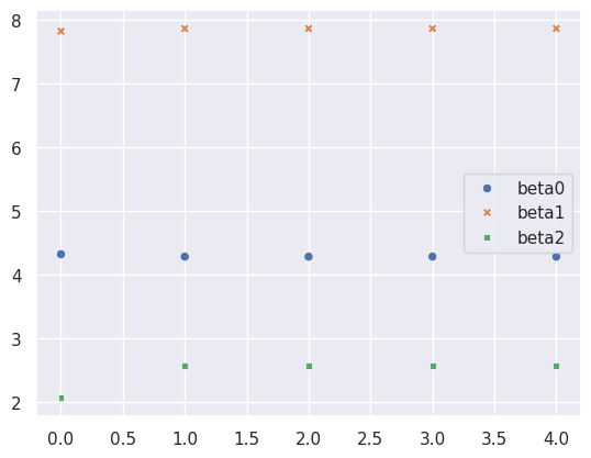
sns.lineplot(df);
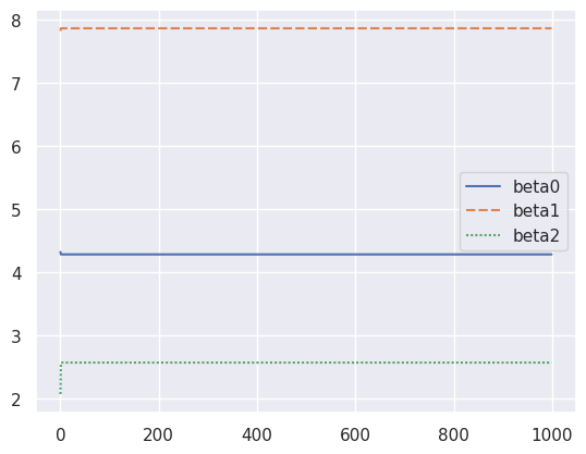
(g)
data = pd.DataFrame({'x1':x1,
                     'x2':x2,
                     'y':y})

X = MS(['x1', 'x2']).fit_transform(data)
results = sm.OLS(y, X).fit()
summarize(results)
| coef | std err | t | P>|t| | |
|---|---|---|---|---|
| intercept | 4.2798 | 0.997 | 4.293 | 0.000 |
| x1 | 7.8606 | 1.095 | 7.181 | 0.000 |
| x2 | 2.5664 | 0.957 | 2.683 | 0.009 |
We’ll compare both methods now.
results.params - [beta0, beta1, beta2]
intercept    3.552714e-15
x1           1.776357e-15
x2          -1.332268e-15
dtype: float64
We can see it’s a very miniscule difference.
fig, ax = plt.subplots()

# Use a fixed palette for consistency between data and baseline lines
palette = sns.color_palette("tab10", n_colors=3)

# Plot the data lines with seaborn. The hue mapping uses our palette.
sns.lineplot(data=df, ax=ax, palette=palette, dashes=False)

# Plot baseline lines for each column in the group.
# Each baseline is drawn as a dashed horizontal line at the coefficient value.
for idx, col in enumerate(df.columns):
    baseline_val = results.params.iloc[idx]
    ax.axhline(y=baseline_val, color=palette[idx], linestyle='--', label=f"Baseline {col}")

ax.legend(loc='upper right', fontsize='small')
ax.set_xlabel('iteration')
ax.set_ylabel('coefficient value')
plt.tight_layout()
plt.show()
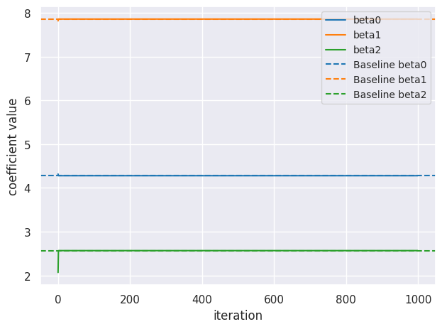
(h)
By iteration 3 the backfitting method was accurate up to 5 significant digits.
np.abs(results.params - df.iloc[2,:].values)
intercept    0.000001
x1           0.000001
x2           0.000014
dtype: float64
And up to around 8 significant digits by iteration 4.
np.abs(results.params - df.iloc[3,:].values)
intercept    5.566243e-09
x1           6.132090e-09
x2           7.371417e-08
dtype: float64
Q12.#
We’ll start by creating 100 predictors \(X_1, ..., X_{100}\) drawn from standard normal distributions and a \(100\) integer coefficients in the range \([-10, 10]\).
I’m setting the sample size \(n = 101\) instead of \(100\) so the matrix does not become saturated and to avoid warnings from sm.OLS later.
n = 101
p = 100
rng = np.random.default_rng(7)
coefs = rng.integers(-10, 11, size=p)
eps = rng.normal(0, 4, size=n)

data100 = pd.DataFrame({f"x{i}":rng.normal(0, 1, n) for i in range(1, p + 1)})
data100.head()
| x1 | x2 | x3 | x4 | x5 | x6 | x7 | x8 | x9 | x10 | ... | x91 | x92 | x93 | x94 | x95 | x96 | x97 | x98 | x99 | x100 | |
|---|---|---|---|---|---|---|---|---|---|---|---|---|---|---|---|---|---|---|---|---|---|
| 0 | -0.694404 | -0.530115 | 0.292268 | -1.085816 | 0.552340 | 0.675451 | -1.084599 | -0.479336 | 0.808410 | 0.884749 | ... | 0.474795 | 1.033411 | 1.076624 | -0.594797 | -0.556457 | 0.353752 | -0.836014 | 1.570142 | -0.222130 | 0.441849 |
| 1 | -0.326685 | 1.333560 | -0.205311 | -0.102069 | -1.664602 | 0.260088 | -0.373664 | 0.938149 | -0.318144 | 0.864653 | ... | 0.146766 | -1.358934 | 0.616559 | 0.043102 | 1.835143 | 0.149400 | 2.312694 | 0.445838 | 0.371477 | 0.649667 |
| 2 | -0.560231 | 0.047120 | 0.214454 | 0.051955 | 0.460453 | -0.922971 | 2.280556 | -0.601504 | 1.855783 | -0.373815 | ... | 1.887452 | 0.405447 | -0.586072 | -0.402486 | -0.248234 | -1.134712 | 1.141353 | -2.202446 | 1.250827 | -0.016700 |
| 3 | 0.007959 | -1.172546 | 0.296739 | 0.958463 | 0.243037 | 0.072866 | -0.069594 | -0.157427 | 1.700440 | -1.117763 | ... | -2.416341 | 0.132935 | -0.576968 | 0.337267 | 1.911494 | 1.170559 | 1.220760 | 1.798199 | -0.577544 | -0.688981 |
| 4 | -0.375267 | -0.940700 | -0.298774 | -0.906269 | 0.283376 | -0.351278 | -0.238661 | 2.486350 | -1.954211 | -1.549745 | ... | -1.545858 | -0.445181 | -0.034345 | -1.334770 | 1.166775 | 0.318499 | -0.356279 | 0.217479 | -0.811713 | -0.006864 |
5 rows × 100 columns
coefs
array([  9,   3,   4,   8,   2,   6,   7,  -6,  -9,  -4,  -5,   8,   9,
       -10,   0,   7,  -8,   6,  -8,  -1,   7,  -4,  -3,  -5,   5,  -5,
        10,  -1,   0,   0,   2,   1,   0,  10,   6,   6,   4,   3,  -3,
        10,  -1,  -6,   7,  -7,   8,   2,  -8, -10,  -1, -10,  -8,   0,
        10,  -1,   6,   9,   7,   3,  -1,   0,  -5,   0,  -3,  -5,  10,
       -10,  -8,  -6,  10,   4,   8,  -6,   5,  -3,   0, -10,   2,   7,
         3,  -7,   1,  -5,  10,   8,  -7,   0,   9,   7,   4,   3, -10,
         5,  -1,  -9,  -5,   1,   5,   0,   2,   8])
Our response \(Y\) will be a sum of all the \(\beta_i X_i\) terms plus a noise term \(\epsilon\).
data100['y'] = data100.dot(coefs) + eps
data100.head()
| x1 | x2 | x3 | x4 | x5 | x6 | x7 | x8 | x9 | x10 | ... | x92 | x93 | x94 | x95 | x96 | x97 | x98 | x99 | x100 | y | |
|---|---|---|---|---|---|---|---|---|---|---|---|---|---|---|---|---|---|---|---|---|---|
| 0 | -0.694404 | -0.530115 | 0.292268 | -1.085816 | 0.552340 | 0.675451 | -1.084599 | -0.479336 | 0.808410 | 0.884749 | ... | 1.033411 | 1.076624 | -0.594797 | -0.556457 | 0.353752 | -0.836014 | 1.570142 | -0.222130 | 0.441849 | -20.430838 |
| 1 | -0.326685 | 1.333560 | -0.205311 | -0.102069 | -1.664602 | 0.260088 | -0.373664 | 0.938149 | -0.318144 | 0.864653 | ... | -1.358934 | 0.616559 | 0.043102 | 1.835143 | 0.149400 | 2.312694 | 0.445838 | 0.371477 | 0.649667 | 6.147675 |
| 2 | -0.560231 | 0.047120 | 0.214454 | 0.051955 | 0.460453 | -0.922971 | 2.280556 | -0.601504 | 1.855783 | -0.373815 | ... | 0.405447 | -0.586072 | -0.402486 | -0.248234 | -1.134712 | 1.141353 | -2.202446 | 1.250827 | -0.016700 | -45.849696 |
| 3 | 0.007959 | -1.172546 | 0.296739 | 0.958463 | 0.243037 | 0.072866 | -0.069594 | -0.157427 | 1.700440 | -1.117763 | ... | 0.132935 | -0.576968 | 0.337267 | 1.911494 | 1.170559 | 1.220760 | 1.798199 | -0.577544 | -0.688981 | 7.119777 |
| 4 | -0.375267 | -0.940700 | -0.298774 | -0.906269 | 0.283376 | -0.351278 | -0.238661 | 2.486350 | -1.954211 | -1.549745 | ... | -0.445181 | -0.034345 | -1.334770 | 1.166775 | 0.318499 | -0.356279 | 0.217479 | -0.811713 | -0.006864 | -87.132218 |
5 rows × 101 columns
data100.describe()
| x1 | x2 | x3 | x4 | x5 | x6 | x7 | x8 | x9 | x10 | ... | x92 | x93 | x94 | x95 | x96 | x97 | x98 | x99 | x100 | y | |
|---|---|---|---|---|---|---|---|---|---|---|---|---|---|---|---|---|---|---|---|---|---|
| count | 101.000000 | 101.000000 | 101.000000 | 101.000000 | 101.000000 | 101.000000 | 101.000000 | 101.000000 | 101.000000 | 101.000000 | ... | 101.000000 | 101.000000 | 101.000000 | 101.000000 | 101.000000 | 101.000000 | 101.000000 | 101.000000 | 101.000000 | 101.000000 |
| mean | -0.188754 | 0.051707 | -0.089834 | -0.342449 | 0.003727 | 0.039669 | -0.168156 | 0.191067 | -0.047862 | -0.030087 | ... | 0.028333 | 0.107951 | 0.127211 | 0.082461 | 0.069857 | 0.059035 | -0.014487 | -0.051020 | -0.029952 | -11.055107 |
| std | 0.977752 | 0.908521 | 0.927207 | 0.888110 | 0.951015 | 1.020977 | 0.957645 | 0.908086 | 0.994167 | 1.044035 | ... | 1.080511 | 1.013363 | 1.052838 | 0.964704 | 1.093956 | 1.132628 | 1.090097 | 0.985822 | 0.982725 | 64.962322 |
| min | -3.251438 | -2.613559 | -1.946678 | -2.819569 | -2.760418 | -2.309521 | -2.100440 | -2.133884 | -2.259497 | -2.405364 | ... | -3.412312 | -2.567531 | -1.749875 | -2.135391 | -2.961898 | -2.804388 | -2.498290 | -2.802652 | -2.062214 | -148.859438 |
| 25% | -0.806846 | -0.555248 | -0.754022 | -0.977258 | -0.600947 | -0.539778 | -0.802186 | -0.457107 | -0.792173 | -0.717843 | ... | -0.701115 | -0.576968 | -0.750318 | -0.556457 | -0.685126 | -0.599964 | -0.649413 | -0.634373 | -0.688981 | -52.681323 |
| 50% | -0.142903 | -0.002029 | -0.132070 | -0.294354 | 0.204663 | -0.068876 | -0.199655 | 0.120471 | -0.070865 | -0.061462 | ... | 0.132935 | 0.198333 | 0.092704 | 0.043114 | 0.160276 | 0.053884 | 0.141063 | -0.214611 | -0.007977 | -13.781208 |
| 75% | 0.493932 | 0.577047 | 0.514521 | 0.091685 | 0.584146 | 0.671333 | 0.435367 | 0.812917 | 0.633794 | 0.647760 | ... | 0.710309 | 0.785195 | 0.985852 | 0.762508 | 0.885498 | 0.694165 | 0.767484 | 0.690311 | 0.590520 | 25.562973 |
| max | 2.025161 | 2.015516 | 2.536930 | 1.908217 | 1.957445 | 2.532306 | 2.571669 | 2.486350 | 2.440462 | 2.508994 | ... | 2.632762 | 2.475546 | 2.491695 | 2.215750 | 2.423589 | 3.632931 | 2.424722 | 2.112505 | 2.632648 | 170.171354 |
8 rows × 101 columns
def simple_reg(outcome, feature):
    y = outcome
    x = feature

    beta1 = np.sum((x - x.mean()) * (y - y.mean()))/(np.sum((x - x.mean())**2))
    beta0 = y.mean() - beta1 * x.mean()
    return beta0, beta1


def backfit(df: pd.DataFrame, response: str, max_iterations=1000):
    X_df = df.drop(response, axis=1)

    iter_dict = {}
    coefs = np.ones(len(df.columns)-1)

    for i in range(max_iterations):
        for j, col in enumerate(X_df.columns):
            # fit model on column j while holding all others constant and ignore the intercept
            _ , coefs[j] = simple_reg(
                    df[response] -  X_df.loc[:, X_df.columns != col].dot(np.delete(coefs, j)),
                    X_df.iloc[:, j]
                )
        iter_dict[i] = coefs

    return iter_dict
backfit_results = backfit(data100, 'y', max_iterations=1000)
final_results = backfit_results[list(backfit_results.keys())[-1]]
final_results
array([ 8.57112098e+00,  3.70741572e+00,  3.47337638e+00,  4.68503048e+00,
        6.24588909e-01,  8.02640881e+00,  4.23987354e+00, -6.03461905e+00,
       -7.06804991e+00, -2.72535620e+00, -6.04071987e+00,  1.03041912e+01,
        1.16840477e+01, -9.25075619e+00,  1.00064332e+00,  9.63917741e+00,
       -7.34386057e+00,  8.85059566e+00, -3.88228087e+00,  3.36003252e-01,
        7.51295395e+00, -4.38840321e+00,  2.08112935e+00,  1.09818560e+00,
        3.67249134e+00, -2.77778291e+00,  8.18339805e+00,  1.79726256e+00,
       -4.30130048e+00,  2.62805183e+00,  2.25731510e-01,  2.26321752e+00,
        1.91491039e+00,  9.20720719e+00,  5.54078131e+00,  6.06956898e+00,
        2.89175935e+00,  6.24697170e+00, -3.70104350e+00,  8.56869727e+00,
        6.72379107e-01, -4.96452568e+00,  8.69038160e+00, -6.79213143e+00,
        4.60505003e+00, -5.77148948e-01, -6.64119591e+00, -9.63568129e+00,
        4.00557815e+00, -6.39587309e+00, -8.88411389e+00, -2.50658472e+00,
        1.17367882e+01,  4.59329264e-01,  9.35473768e+00,  1.09809613e+01,
        7.27130949e+00,  6.15605252e+00, -7.16367036e-03,  2.00043013e+00,
       -8.76106236e+00, -9.15577933e-01, -3.91496094e+00, -3.12776996e+00,
        1.00526512e+01, -1.04172173e+01, -4.12726618e+00, -4.53944208e+00,
        8.60869014e+00,  1.89162776e+00,  1.19969255e+01, -3.33042320e+00,
        4.96087267e+00, -8.33321737e-01,  9.19303135e-01, -1.07399984e+01,
        3.29317513e+00,  2.10660948e+00,  6.22367954e+00, -1.58239828e+00,
        3.81631058e+00, -2.38955632e+00,  1.15056470e+01,  6.81957089e+00,
       -6.74912212e+00, -3.30772445e+00,  7.02509480e+00,  8.48840876e+00,
        1.62145940e+00,  4.00581560e+00, -1.06914126e+01,  4.29738267e+00,
        1.08705114e+00, -9.07482450e+00, -4.81436886e+00,  2.91526891e+00,
        3.86411031e+00,  2.35734324e+00,  8.65347733e-01,  1.06290876e+01])
We’ll check on the \(\text{MAE}\) between the coefficients we got and the true underlying coefficients.
np.mean(np.abs(coefs - final_results))
1.865078631822381
Which is not bad considering the \(\text{mean}\) and \(\text{stddev}\) of the true coefficients.
coefs.mean(), coefs.std()
(0.72, 6.110777364623915)
backfit_df = pd.DataFrame.from_dict(backfit_results, orient='index')
backfit_df.columns = data100.columns.drop('y')
backfit_df.head()
| x1 | x2 | x3 | x4 | x5 | x6 | x7 | x8 | x9 | x10 | ... | x91 | x92 | x93 | x94 | x95 | x96 | x97 | x98 | x99 | x100 | |
|---|---|---|---|---|---|---|---|---|---|---|---|---|---|---|---|---|---|---|---|---|---|
| 0 | 8.571121 | 3.707416 | 3.473376 | 4.68503 | 0.624589 | 8.026409 | 4.239874 | -6.034619 | -7.06805 | -2.725356 | ... | -10.691413 | 4.297383 | 1.087051 | -9.074825 | -4.814369 | 2.915269 | 3.86411 | 2.357343 | 0.865348 | 10.629088 |
| 1 | 8.571121 | 3.707416 | 3.473376 | 4.68503 | 0.624589 | 8.026409 | 4.239874 | -6.034619 | -7.06805 | -2.725356 | ... | -10.691413 | 4.297383 | 1.087051 | -9.074825 | -4.814369 | 2.915269 | 3.86411 | 2.357343 | 0.865348 | 10.629088 |
| 2 | 8.571121 | 3.707416 | 3.473376 | 4.68503 | 0.624589 | 8.026409 | 4.239874 | -6.034619 | -7.06805 | -2.725356 | ... | -10.691413 | 4.297383 | 1.087051 | -9.074825 | -4.814369 | 2.915269 | 3.86411 | 2.357343 | 0.865348 | 10.629088 |
| 3 | 8.571121 | 3.707416 | 3.473376 | 4.68503 | 0.624589 | 8.026409 | 4.239874 | -6.034619 | -7.06805 | -2.725356 | ... | -10.691413 | 4.297383 | 1.087051 | -9.074825 | -4.814369 | 2.915269 | 3.86411 | 2.357343 | 0.865348 | 10.629088 |
| 4 | 8.571121 | 3.707416 | 3.473376 | 4.68503 | 0.624589 | 8.026409 | 4.239874 | -6.034619 | -7.06805 | -2.725356 | ... | -10.691413 | 4.297383 | 1.087051 | -9.074825 | -4.814369 | 2.915269 | 3.86411 | 2.357343 | 0.865348 | 10.629088 |
5 rows × 100 columns
X = MS(data100.columns.drop('y'), intercept=False).fit_transform(data100)
results = sm.OLS(data100['y'], X).fit()
summarize(results)
| coef | std err | t | P>|t| | |
|---|---|---|---|---|
| x1 | 8.9331 | 7.355 | 1.215 | 0.438 |
| x2 | 4.7279 | 4.561 | 1.037 | 0.489 |
| x3 | 4.4370 | 4.725 | 0.939 | 0.520 |
| x4 | 5.3049 | 5.407 | 0.981 | 0.506 |
| x5 | 0.7438 | 4.395 | 0.169 | 0.893 |
| ... | ... | ... | ... | ... |
| x96 | 0.4842 | 3.387 | 0.143 | 0.910 |
| x97 | 4.5245 | 6.536 | 0.692 | 0.615 |
| x98 | 0.3164 | 4.599 | 0.069 | 0.956 |
| x99 | 2.2474 | 9.718 | 0.231 | 0.855 |
| x100 | 7.6208 | 10.415 | 0.732 | 0.598 |
100 rows × 4 columns
results.params[results.pvalues <= 0.05]
Series([], dtype: float64)
The t-statistics and p-values aren’t significant mostly because there’s only 1 degree of freedom to calculate them \(n = 101, p = 100\).
We can see that the \(\text{MAE}\) for the coefficients of the multiple regression model and the ones we got using backfitting isn’t that big.
np.mean(np.abs(results.params - final_results))
1.5048746861790105
We’ll split the 100 predictors on 20 plots 5 predictors each, we’ll use solid lines for the backfitted coefficient values and dashed lines for the coefficients obtained from the multiple regression and label them as Baseline.
# Create a 5x4 grid of subplots (20 subplots total)
fig, axes = plt.subplots(5, 4, figsize=(20, 25), sharex=True, sharey=True)
axes = axes.flatten()

n_groups = 20
cols_per_group = 5

for i in range(n_groups):
    start = i * cols_per_group
    end = start + cols_per_group
    subset = backfit_df.iloc[:, start:end]

    # Convert the subset to long format to easily plot with seaborn and retain legend
    subset_long = subset.reset_index().melt(id_vars='index', var_name='Coefficient', value_name='Value')

    # Use a fixed palette for consistency between data and baseline lines
    palette = sns.color_palette("tab10", n_colors=cols_per_group)

    # Plot the data lines with seaborn. The hue mapping uses our palette.
    sns.lineplot(data=subset_long, x='index', y='Value', hue='Coefficient', ax=axes[i], palette=palette)

    # Plot baseline lines for each column in the group.
    # Each baseline is drawn as a dashed horizontal line at the coefficient value.
    for idx, col in enumerate(subset.columns):
        baseline_val = results.params.iloc[start + idx]
        axes[i].axhline(y=baseline_val, color=palette[idx], linestyle='--', label=f"Baseline {col}")

    axes[i].set_title(f"Columns {start+1} to {end}")
    axes[i].legend(loc='upper right', fontsize='small')

plt.tight_layout()
plt.show()
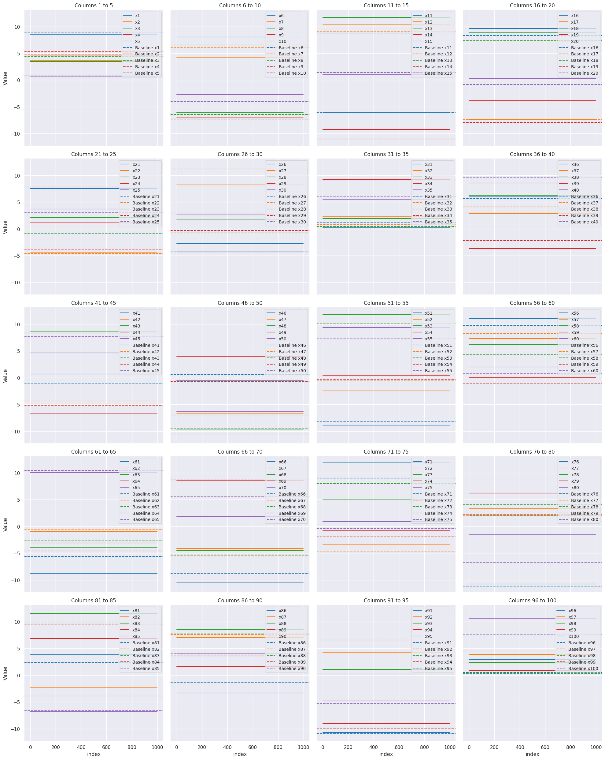
Looking at the plots above we can see that a lot of backfit approximated coefficients fall pretty close to the baseline set by multiple regression.
And that it converged in around 2 or 3 iterations even though we had \(100\) predictors.